Historical Data Analysis and Forecast for Demand

Introduction

Demand forecasting is essential for any business as it allows for making informed financial decisions and managing risks. According to Taghipour (2020), forecasting techniques determine production needs, and the use of time series can help in identifying a seasonal component. In the given scenario, KTP company operating in the tires industry reported its historical series of sales to get an evaluation of seasonality’s impact on its business (Genovese & Simpson, 2016). KTP produces tires for agricultural machines, primarily for vineyard tractors. No major changes are expected in the business climate and industrial operations in the short term. The purpose of this paper is to analyze the historical data of KTP, identify the appropriate forecasting method, and calculate a forecast for the overall demand for the next year, providing recommendations for the company.

Analysis of the Historical Data

To begin with, a time series for the KTP company’s historical data were plotted, as depicted in Figure 1. As can be seen, there is a strong seasonal component that allows for identifying a recurrent demand pattern within a year, with a peak in August and a valley in February (see Fig. 1). The seasonality of the agricultural industry has a significant impact on the KTP company’s sales. In addition to the cyclic movement of the historical data, the overall trend of the plot is increasing.

Given the seasonal nature of the KTP company, the use of the deseasonalization technique can prove effective for demand forecasting. To apply the deseasonalization technique, a number of steps were implemented, as discussed below. The Moving Average (MA) and Centered Moving Average (CMA) were calculated for the historical data to eliminate the seasonal and irregular components. Then, the CMA was plotted, as presented in Figure 1. The seasonal (S_t) and irregular (I_t) components were identified to deseasonalize the data. The next step was to determine the trend component (T_t) in order to apply the following multiplicative model formula: Y_t = S_t * I_t * T_t (Russell & Taylor, 2019). Excel’s Data Analysis Toolkit was utilized to obtain simple linear regression output and identify the coefficients required to calculate the trend component. Consequently, the forecast for the historical data was calculated using the formula Forecast = S_t * T_t. Year 4 sales predictions were created, as presented in Table 1. As shown in Figure 2, the historical data with actual values and the forecast with predicted values including Year 4 are well approximated.

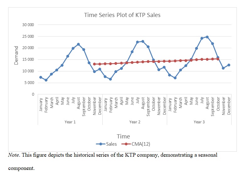
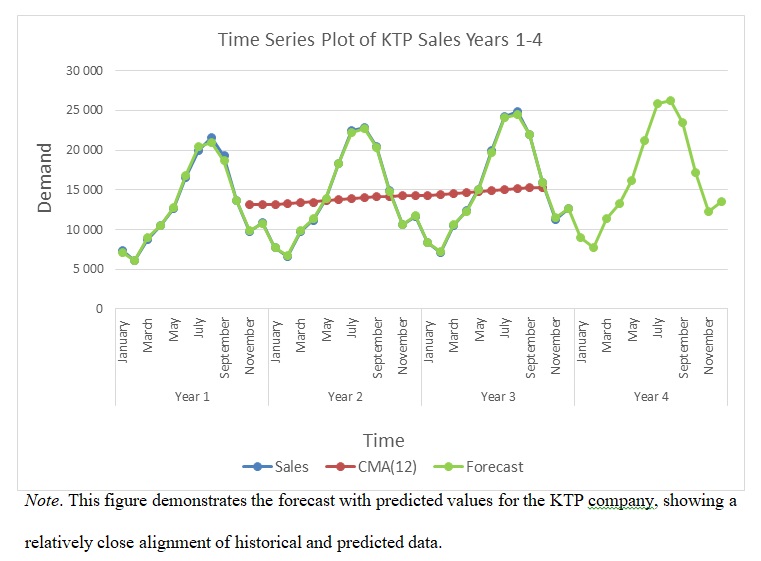
Table 1. Forecast for KTP for Year 4.

Note. This table depicts the forecasting data for Yeat 4 of the KTP company, obtained through the use of the deseasonalization technique.

Conclusion and Recommendations

To conclude, the application of the deseasonalization method to the given scenario and historical data allowed for generating a reliable forecast for Year 4 for KTP. The company can use the predicted values provided that no major changes happen in the market and the agricultural industry. Due to the limitations associated with the forecast, it is recommended to ensure that an analysis of broader conditions is conducted. Overall, KTP can use the forecast to enhance its production and planning activities.

References

Genovese, A., & Simpson, M. (2016). KTP tyres: The use of deseasonalization techniques in demand forecasting. Kogan Page Case Study Library EAN 9780749477820. Web.

Russell, R. S., & Taylor, B. W. (2019). Operations and supply chain management (10^th ed.). John Wiley & Sons.

Taghipour, A. (2020). Demand forecasting and order planning in supply chains and humanitarian logistics. IGI Global.