Saudi Arabia: Linear and Non-Linear Techniques for Estimating the Money Demand Function

intertemporal utility over a finite planning horizon of T periods, in each period. The consumer’s intertemporal utility function isAbstract

The main objective of this research study is to estimate and analyze the money demand function in Saudi Arabia applying two different approaches. The conventional way is based on non-oil GDP measures for income. The second, the consumer demand theory, is based on microeconomic and aggregation theory which involves monetary assets as durable goods, which are directly impeded in the household utility function. To prove the validity of the results Simple-Sum (M1, M2) and Divisia (M1, M2) are used. Two techniques, Cointegration and Error-correction and Back Propagation Neural Network are employed to estimate the money demand function. To analyze the different monetary aggregates, the cointegration method is used. The paper uses Divisia monetary aggregates M1 and M2 outperformed the Simple-Sum M1 and M2 for long-run money demand function analysis. Changes in interest rates exert obvious pressure on speculative holdings of cash balances or those simply having a strong taste for highly liquid asset portfolios. More attractive yields encourage ventures farther out on the liquidity spectrum. The money demand function affects desired ordinary transactions balances. At higher interest rates, firms have a greater incentive to invest funds that have piled up under the aegis of favorable cash flows; funds awaiting dispersal later in the receipts-disbursements cycle. Inconvenience and frictional expense seem less important with the increased opportunity cost of holding cash. Similarly, even if payments periods were unaffected by changed interest rates, households (et al.) would be spurred by higher interest rates to place idle funds in securities while awaiting the active phase of their expenditure cycle. The results obtained from the consumer demand theory approach indicate a significant role for the opportunity-cost variable that conforms to the theory when Divisia dual price is used as the opportunity-cost variable in the money demand function.

Introduction

Money market activity and the lightning speed at which funds can now quit countries has prompted many commentators to question its worth and, in light of heightened vulnerability to foreign investor sentiment, to emphasize its perceived dangers. In particular, strong objections to the ever-increasing trend of financial globalization have been raised because the governments of the economies most affected have ceded their economic sovereignty to international investors. Accordingly, it is said that the priorities and policy choices facing national governments can no longer be considered and implemented without first taking possible foreign investor reactions into account. Yet it can be shown that financial globalization tends to improve, rather than worsen, a nation’s overall economic welfare and that having an internationally integrated economy provides a safeguard against irresponsible growth limiting and inflationary policies. Over recent decades, funds have mostly flowed across country borders as bank lending or to acquire debt instruments, although considerable foreign equity investment has also occurred, especially after the privatization of state enterprises in many economies. The macroeconomic significance of international financial flows and external payments imbalances critically depends on prevailing exchange rate arrangements, as well as the extent of official restrictions in the form of capital controls. To put the existing global financial system in a historical context, it is necessary to consider the evolution of the international monetary and financial system.

The paper aims to apply linear and non-linear techniques for estimating the money demand function in Saudi Arabia. Special attention is given to the theory of Divisia Monetary Aggregation. The research is based on the empirical methodology which includes a model that is consistent with the principles of microeconomic and aggregation theory. The case study is constructed by the index numbers and methods derived from economic theory. Also, a system of equations that models the wealth holder’s allocation of total expenditures between money and non-money assets are used. The Johansen cointegration technique and error correction models are used to determine and analyze the long-run and short-run concepts of the demand for money in Saudi Arabia in both approaches.

In Saudi Arabia, the fundamental causes have internationalized production and finance – improvements in technology and the liberalization of markets for goods, services and savings. Technological advances in electronics have greatly reduced the costs of communication and computing, conquering the natural barriers of time and distance. Since that time, the invention of computing and new ways of instantly transmitting information around the world in print forms, such as by facsimile, email and the internet have reconstructed international communications. More generally, computers have revolutionized the processing and dissemination of information, its use greatly encouraged by the fact that since the mid-1970s the cost of computer processing has been falling by an average of 30 percent per year in real terms. Within the open economy models, some authors have recognized a role for the current account in terms of its implications for the international investment position and hence for financial wealth holdings. The intertemporal approach to foreign investment provides a basis for introducing offer curves, usually only employed in the pure theory of international merchandise trade, to model the external accounts. Casting the intertemporal approach in terms of offer curves serves to highlight that, contrary to the approaches to the external accounts. Despite popular assumptions to the contrary, while respecting traditional beliefs and values, Saudi Arabia has been able to effect substantive change and reform. Modernization is not being questioned; false models and false friends are being questioned. Here it is assumed that the substitution effect on present consumption of an interest rate change at least offsets any income effect. Even if the income effect dominated the substitution effect, however, offer curves can still be constructed, provided the extra investment stemming from the lower interest rate exceeds any additional consumption in the first period. In parallel with orthodox international trade theory, the offer curves demonstrate that when foreign investment is allowed and capital markets are fully integrated, a common price, the return on capital, Foreign investment confers welfare gains if economies’ real interest rates would be different without trade. Economies would not engage in intertemporal trade, however, irrespective of the extent of capital mobility, if domestic interest rates were identical in autarky.

Linear and non-linear techniques are used to analyze money supply and determine current monetary issues in Saudi Arabia. The abolition of official restrictions governing cross border transactions over recent decades has transformed the financial markets of many economies from being heavily regulated and segmented, into ones that are lightly regulated and more internationally integrated. Access to international financial capital and services has increased greatly which has boosted borrowing and lending opportunities and enhanced capital mobility. Whereas much of the foregoing analysis focused on international flow magnitudes, this section shifts attention to aggregate stocks to model the stock adjustment effects of international financial liberalization. In particular, it shows how financial globalization may affect a nation’s external indebtedness position, as well as the value of its capital stock and wealth. In a certain world with a competitive capital market and no transactions costs, the present value of firms’ investment is also the market value of the firms’ common shares, which in this simple model equals the value of the economy’s assets. Optimal investment decisions by firms maximize the net present value of investments and also maximize the value of national assets. The paper consists of an introduction, five chapters and a conclusion.

Chapter one

Overview of Saudi Arabian Economy

As a country, Saudi Arabia possesses three distinct characters; as a strong and independent Arabic country; as the country that provides a home for the two holiest Muslim cities; and as the single largest producer of oil in the world. On the economic front, it is the oil reserves of the country, which have turned this desert nation into one of the strongest economies of the world. It was due to the relentless efforts of the House of Saud from the year 1902 until 1932 that unified the tribes of the desert nation against the colonial powers of the United Kingdom and France. These efforts led to the creation of Saudi Arabia as an independent nation under the guidance and steering by the House of Saud as the country’s royal family. Many of the prominent Saudis have sent their sons to the United States and Western countries to study and these people have brought Western economic thoughts back into the country. With the economic ideas brought in by these people, the extremely religious society has turned slowly into one of the progressive economies of the world. This chapter briefly outlines the background of the Saudi economy and the financial system prevailing in the country along with the monetary policies implemented in the country.

Background and Overview of the Economy

With a view to encourage the inflow of foreign direct investments into the country, the government set up the Saudi Arabian General Investment Authority in the year 2000. However, the country continued its restrictive policies in respect of certain industries. As an integral part of the economic reforms instituted by the country, the government decided to get the accession into the World Trade Organization (WTO) in the year 2005. These steps taken by the Saudi government has accelerated the economic growth to reach an average of over 5 percent in the last few years. The economic growth is in tandem with the increase in demand for oil and other petroleum products throughout the world. Because of the economic growth, the country has also become one of the active investors in other countries of the world.

Despite the rapidity of the economic growth, there are major challenges that the country faces; like the aquifer depletion and the increased cost of water supply. Continued dependence on oil and political instability in the Middle East are some of the other issues that draws the attention of the country away from the economic progress. Demographic factors also cause serious concern in the economic outlook of the country with 40% of the population with an average age of 15 or less, low education and higher unemployment levels. These issues are likely to result in major social unrests.

The Saudi Arabian economy is oil-based with the government having a strong control over major economic activities of the country. The country is in possession of more than 20% of the world petroleum reserves and is the largest exporter of oil mainly to United States and many other countries. The country is an active member of Organization of Petroleum Exporting Countries (OPEC), and plays a leading role in the activities of OPEC. As of May 2008 75% of Saudi’s budget revenues is contributed by petroleum sector and 45% of the Gross Domestic Product (GDP). During the same period, 90% of the export earnings are from petroleum exports. The country has an expatriate population of about 5.5 million workers who contribute to the development of the economy.

Increase in oil prices and the macroeconomic and structural reforms undertaken by the country enabled Saudi Arabia to accelerate the momentum of its economic growth. The economic reforms measures were undertaken by the government to support the comprehensive and sustainable economic development in all the economic and social areas of the country. The continued increase in oil prices until mid 2008 coupled with the supportive actions initiated by the government witnessed an all round improvement in the performance of all sectors of the economy. The overall GDP registered a growth of 7.1 percent in current prices (Riyals 1.4 trillion) and 3.4 percent in real terms (Riyals 813.0 billion) for the year 2007. There was a surplus in the State budget to the extent of 12.3 percent of GDP (Riyals 176.6 billion) as against the surplus of 21 percent (Riyals 280.4 billion) for the previous year. The country had a very favorable balance of payments position for the consecutive ninth year with a surplus of Riyals 356.3 billion registering a decline of 4.0 percent as against that for the year 2006. Some of the economic indicators are presented in the table below:

Selected Economic Indicators

Source: Annual Report of SAMA

Economic Growth

Central Department of Statistics and Information (CDSI) has reported a growth in the GDP at current prices of 7.1 percent for the year 2007 while, the non-oil sector grew by 4.5 percent to 840.4 billion Riyals for the same year. The contribution by non-oil sector contributes about 45.6 percent of the total GDP. The growth in non-oil private sector GDP was in the region of 8.0 percent at 403.8 billion Riyals as compared to that of government non-oil sector growth of 4.2 percent, which in real terms accounted for 228.9 billion Riyals. The oil-sector registered a growth of 8.0 percent with 778.4 billion Riyals constituting 54.4 percent of the total GDP at current prices.

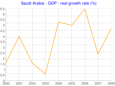
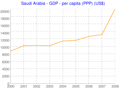
The real growth rate of GDP and the per capita GDP for the country is presented in the following tables and diagrams:

GDP – Real Growth Rate

Per Capita GDP

Inflation Rates

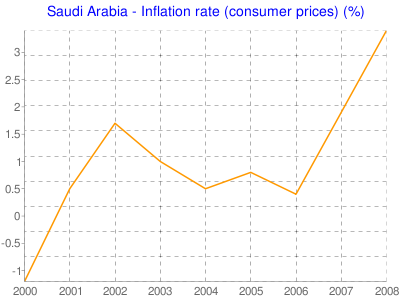
The general cost of living for all the cities registered an increase of 4.1 percent in 2007 (1999=100) and the wholesale price index showed an increase of 5.7 percent for the same year. There was an increase of 15.2 percent in the total supply for goods and services in the year 2007. At the same time, the total demand for goods and services registered a growth rate of 12.9 percent (Saudi Arabian Monetary Agency, 2008).

There was an annual increase of 40.9 percent in the general share price index to reach the position of 11,176 points as at the end of the year 2007 as compared to 7933.9 points as at the end of 2006. Market capitalization of issued shares increased to the level of Riyals 1949 billion in the year 2007 from the position of 1,226 billion as of 2006 (Saudi Arabian Monetary Agency, 2008).

Banking sector registered an impressive growth in the year 2007 with the rise in the deposits to 21.4 percent to Riyals 717.6 billion. This increase compares with the increase of 20.8 percent for the year 2006. Bank deposits accounted for 90.9 percent of aggregate money supply at the end of the year 2007 as against 89.5 percent as at the end of the year 2006 (Saudi Arabian Monetary Agency, 2008).

According to the estimates presented by Central Department of Statistics and Information, the population of the country stood at 24.24 million in the year 2007, out of which Saudis were 17.7 million constituting 73.0 percent of the total population. Non-Saudis were about 6.5 million representing 27.0 percent of the population. As per the statistics provided by the Ministry of Labor for the year 2007 the total labor force working for the private sector was about 5.8 million and out of this 13.1 percent only were Saudis and the balance of 86.9 percent represented non-Saudis. This shows the excessive dependence of the private sector on the expatriate labor force. However, the statistics presented by Ministry of Civil service indicate the total number of work force working for the government at 830,000 of which 91.7 percent are Saudi nationals and non-Saudis are a meager percentage of 8.3 only. The Saudi male workers working for the government of the Kingdom were 508,000 and the Saudi female workers are 253,000 (Saudi Arabian Monetary Agency, 2008).

On the fiscal side the actual revenue and expenditure for the fiscal year corresponding to the calendar year 2007 has indicated a decline of 4.6 percent in the actual revenues at Riyals 642.8 billion as against the previous year revenue of Riyals 673.7 billion. However, the actual expenditure has gone up by 18.5 percent during the fiscal year to Riyals 466.2 billion whereas the expenditure for the year 2006 was Riyals 393.3 billion. Actual surplus was in the region of Riyals 176.6 billion for the year 2007 as compared to the surplus in the year 2006 of Riyals 280.4 billion. Oil revenues accounted for 87.5 percent of total revenues in the year 2007. The current account surplus was Riyals 356.3 billion in the year 2007 (Saudi Arabian Monetary Agency, 2008).

Financial System in Saudi Arabia

Medium term strategies in respect of economic diversification and acceleration to the economic growth are greatly facilitated by the financial reforms undertaken by any economy. The financial system of Saudi Arabia is quite diverse as compared to that of other economies in the region. Considering the international standards, the banking sector in Saudi can be termed as modest in size with the bank deposits constituting 90.9 percent of the money supply as at the end of the year 2007. The commercial banks claim in the domestic private sector amounted to 557.9 billion Riyals as at the end of the year 2007 recording a growth of 21.4 percent.

The financial system operating in the economy of Saudi Arabia is bank centric with the assets of commercial banks account for 1075.2 billion Riyals which increased by 24.9 percent in the year 2007. All the commercial banks are licensed to operate internationally and they can manage mutual investment funds on their own. Public ownership is found to be extensive. Five banks had more than 20 percent of the holding by public and one bank had the public holding of more than 70 percent. There is participation from the foreign banks and the participation is through significant equity contributions. Six banks are found to have more than 20 percent of foreign equity.

In terms of assets size the non-bank portion of the financial system is dominated by quasi-financial institutions of which the largest are represented by three is Autonomous Government Institutions (AGI). These AGIs dominate the primary market for the government securities. They are authorized to hold wide range of domestic and foreign investments. Saudi Arabian Monetary Agency (SAMA) the apex banking institution of the country manages some of these institutions. There are specialized credit institutions extending interest free loans to priority sectors like housing, agriculture or specific industrial needs. The operations of these institutions are controlled by board of directors appointed by the Council of Ministers. The GOSI and the Pension Fund representing the AGIs and the Public Investment Fund (representing specialized credit institution) hold equity ownership in some of the commercial banks. Public Investment Fund has a large ownership in Saudi Commercial Bank. However, the nonbanking financial sector in Saudi Arabia is in the development stage with leasing companies, insurance companies and licensed moneychangers accounting for a meager percentage of less than one in the total financial system assets (IMF Country Report, 2006).

The banking system in Saudi Arabia is regulated by three distinct factors; the banking assets are funded largely by deposits in the nature of low-cost demand deposits that account for more than 40 percent of total deposits. The low cost deposits when used to lend at interest rates comparable to the international level consistent profitability for the banks. Secondly, the excessive dependence on oil revenue sources makes it difficult for the banks to attempt for any risk diversification domestically more particularly credit risk. Diversifying credit risk necessitates a high level of capital requirement and provisioning which deters the efforts of banks in the direction of diversifying domestically. Thirdly, banks work on extremely conservative lending policies. Such policies prescribe limits for lending to various sectors, limitations on lending to connected parties, prescription of liquid asset ratios, and approval from SAMA for foreign lending and imposing of limits on individual indebtedness. This promotes a managed risk environment and coupled with advanced asset-liability management the banks are able to ensure stability in the financial system. However, the intermediation by commercial banks remains modest only (IMF Country Report, 2006).

The financial system of Saudi Arabia has been structured to have multi-layers expected to play significant role in economic, exchange and regulatory areas. Saudi Arabian Monetary Agency (SAMA) has been placed at the top of the system as the apex institution and SAMA is entrusted with setting the overall monetary policy of the country. Other functions of SAMA include securing the stabilization of the currency value amidst economic openness in exchange transactions and capital flows. SAMA makes use of a number of monetary policy instruments for this purpose. Such policy instruments include setting of the interest rates close to comparable dollar rates for the commercial banks, monitoring and control of foreign assets and introduction of medium-term and short-term government papers to effectively control the budgetary and balance of payments position and to efficiently control the fluctuations in domestic liquidity. SAMA acts as the regulator of all commercial banks, exchange dealers and moneychangers. It is also the depository of all government funds. SAMA disburses funds for purposes approved by the minister of finance for improving national economy (Metz, 1992).

Broad money (M3) consisting of currency outside the banking system and bank deposits recorded an increase of Riyals 129.2 billion representing 19.6 percent and the total deposits stood at Riyals 789.8 billion in 2007. This compares with a rise of Riyals 106.9 billion and the percentage increase was 19.3 in 2006. The increase in M3 was due to growth in bank claims on the private sector. This increased by 21.4 percent. Substantial growth in net domestic expenditure of the government also contributed to the increased broad money situation. The government increased its expenditure outlay on several development projects and social services during the year 2007. The continued increase in imports that created a large deficit in the balance of payments of the private sector greatly neutralized the impact of the expansionary effect of increase in net domestic government expenditure and the increased claim of the banks on the private sector (Saudi Arabian Monetary Agency, 2008).

Conduct of Monetary Policy in Saudi Arabia

Exchange rate has a dominant role to play in most of the economies of emerging countries than the interest rate mechanism. This is due partly to the lesser development of domestic banking systems in these countries and partly due to the fact that full range of monetary instruments is not prevalent in these countries. The exchange rate influences the transmission mechanism by affecting the aggregate demand through the net exports and by affecting the inflation rate through the pass-through effect. During recent periods, the monetary policy in the Kingdom of Saudi Arabia has been subjected to the influence of abundant liquidity resulting from higher oil prices. The monetary policies are also influenced by the increased consumer and business lending by the domestic banks. The formulation of monetary policies in the country is subject to meeting the challenge of asset price inflation and providing wide range of financial assets to domestic banks to extend the area of operation of transmission mechanism. There is the increased focus on Islamic financing principles also (Al-Jasser & Banafe).

The monetary policy framework of Saudi Arabia is based on a fixed exchange rate policy. The country uses the exchange rate mechanism as the nominal anchor for keeping the inflation rate low and for facilitating the stability of exchange rate expectations. Due to the linking of the inflation with the exchange rate, there is the increased public confidence in the monetary policy framework. This also enlarges the opportunities for increased inflow of foreign capital for domestic investments. Since the external receipts and payments of the country are predominantly in US dollars the country adopts the policy of pegging the Saudi Riyal against US dollars. Further most of the oil revenues are subject to variations due to changes in world oil demand. Therefore, the variations in the revenue do not allow the country to adjust the exchange rates according to these variations. To mitigate this shortcoming the government attempts to stabilize the economy by adopting a counter-cyclical fiscal policy. Under this policy, the government strives to keep the expenditures steady in the wake of volatility in the receipts. Hence, the stability of the exchange rate for Saudi Riyal against US Dollar becomes critically important in framing the overall economic policies of the country. US Dollar is therefore the anchor and intervention currency for the Riyal (Al-Jasser & Banafe).

The monetary policy of Saudi Arabia consists of different elements; (i) policy targets, (ii) strategy, (iii) operational framework, and (iv) transmission mechanism. Policy target determines the broad outlook of the monetary policy like for example whether to pursue medium-term price stability or stability in exchange rates. Based on strategies the government determines the levels of interest rates the government wants to achieve over the period. Operational framework enables the government to embark on the ways in which the required interest rate levels can be achieved by using the available instruments like repo rates and adjustment of reserves. Monetary policy transmission mechanism is the process through which the policy decisions are implemented to influence the economy generally and to achieve the policy targets in particular.

The government uses rules targeting inflationary tendency, exchange rate, monetary aggregates and the levels of bank reserve as some of the policy strategies. These strategies have the ability to limit the discretion of the central bank and to enhance its credibility. Through these strategies, the government is able to anchor the expectations of private sector effectively (Al-Jasser & Banafe).

In the Saudi Arabian context exchange rate has been a predominant factor in conducting the monetary policies of the government. In the past reserve, requirements have been the major monetary policy instrument. However, SAMA has not gone in for any changes in reserve requirements since the year 1980. After the passing of the Central Bank Bills in the year 1984,

In an economy controlling its monetary policies through fixed exchange rate mechanisms with perfect asset substitutability as in the case of Saudi Arabia, monetary policy cannot be found to be autonomous. Especially in the context of Saudi Arabia, the oil revenues and their predominant impact on setting the fiscal policy will greatly influence the framing of monetary policies. SAMA has adopted a policy of passive accommodation of system liquidity and that of non-interference with the free operation of the market mechanism. As far as the asset price inflation is, concerned SAMA continues to behave extremely cautious on targeting asset prices due to the reason that asset price valuation has always been a complex phenomenon and is challenging.

SAMA has been using repo rates as the single policy instrument for monitoring the liquidity in the day-to-day system changes and in arriving at the desired overnight rate to the market. Government Development Bonds became a part of the government debt market in the year 1988 and the Treasury Bills were replaced by the Central Bank Bills in the year 1992. Presently SAMA uses the repo rates and reverse repo rates as the effective instruments for conducting the monetary policy of the country. The recently generated budget surpluses have enabled the government to repay longer-dated government debts. However, in order to ensure that the repo rate mechanism is not hampered SAMA takes care that adequate Treasury Bills are in circulation in the market. Whenever there are more speculative activities in the forward market against Saudi Riyal, SAMA intervenes in the forward market by its repo rate policy to contain wide variations in exchange swap points and interest rates. In all respects SAMA maintains the formulation of monetary policy unhindered by its role as debt manager of the government. The monetary policies in general are formulated in response to overall macroeconomic considerations (Al-Jasser & Banafe).

During the year 2007 SAMA continued its endeavour its control on monetary policy aimed to achieve the objective of maintaining stability in domestic prices as well as to maintain the exchange rate for Saudi Riyal. The objective behind the efforts of SAMA is to encourage investments and to increase the competitiveness of the Saudi economy. SAMA had to undertake the challenge of conducting the domestic economic and monetary policies in the direction of harmonizing the spending requirements for development purposes. This is necessary to bring diversification in the economic advancement of the nation and to create more job opportunities. Such policy measures are also aimed at reducing the inflationary pressures. In order to achieve the required results SAMA increased the repo rate by 30 basis points from 5.20 percent to 5.50 percent during the first quarter of 2007. During the same period the reverse repo rates were raised from 4.70 percent to 5.00 percent by 30 basis points. In the last quarter of 2007 SAMA has reduced the repo rates several times up to 100 basis points to bring the rate up to 4 percent. This action from SAMA was necessary to bring stability in the domestic currency. The statutory deposit percentage in respect of demand deposits of commercial banks was raised from 7.0 percent to 9.0 percent in November 2007 (Saudi Arabian Monetary Agency, 2008).

Plan of Dissertation

In order to make a comprehensive presentation the dissertation is structured to have different chapters. While the introductory chapter discussed the background and the overview of the Saudi economy including the financial systems and conduct of monetary policies in the country, chapter two deals with the theoretical aspects of Divisia Monetary Aggregation. This chapter presents the process of constructing Divisia Monetary Aggregates for Saudi Arabia and compares Simple-sum and Divisia Monetary Aggregates for the country. Chapter three contains a detailed review of the literature on the theoretical aspects of demand for money in general with different approaches to the demand for money explained vividly. Part of this chapter discusses the salient aspects of money demand in the context of Saudi Arabia. Chapter four contains a detailed description of the hypothesized models and the methodology followed for completing this study. This chapter details the process of the two alternative techniques of linear (co-integration and Error-correction) and non-linear (Back Propagation Neural Network) which are used in the estimation of demand for real money in the short and long run money demand functions. An empirical analysis of the methods adopted by the study is presented as chapter five. Few concluding remarks summarizing the objective and accomplishments of the study is presented at the end, which marks the end of the dissertation.

Chapter tw0

Divisia monetary aggregates

Introduction

Monetary aggregates are crucial and commonly used as the measure for money in most of the macroeconomic and monetary models. They can be a useful instrument of monetary policy. Moreover, monetary aggregates do help in explaining the behavior of the economic agents. This suggests that constructing appropriate monetary aggregates is crucial. However, the simple-sum monetary aggregates, which are simply summing monetary assets assuming perfect substitution, are the most commonly adopted by central banks around the world; hence, researchers have only those aggregates to use in their studies unless they spend a considerable time to construct their own aggregates.

At least two widely recognized theoretical deficiencies are emphasized in regard to validity of the official simple-sum aggregates. The first criticism concerns the collection of monetary assets comprising aggregates. The simple-sum aggregates are basically ad hoc bundles of monetary assets. Theoretically, to be an optimal aggregate, a monetary aggregate must contain a linearly homogeneous and weakly separable bundle of monetary assets.¹ That is, a set of component monetary assets, M, is an optimal aggregate if the elasticity of substitution between any component asset in M and any asset not in M is independent of the quantity of any asset not in M. This restriction implies the weakly separable condition that the marginal rate of substitution between any two assets in M is independent of the quantity of any asset not in M.

The second defect with the simple-sum aggregates is the method used for aggregating over different components. The simple-sum aggregates are created by simply adding together the nominal values of each component included in the aggregate and assigning them an equal (unitary) weight. That is:

where x_i is the i^th monetary component of subaggregate M1 and n is the number of monetary assets. This form of aggregation assumes that the components are perfect substitutes for each other as money on a one-for-one basis. If this were the case, then the economic agent would hold only the one with the lowest opportunity cost (corner solution case). Furthermore, simple-sum aggregates can not internalize pure substitution effect.

The shortcomings of the simple-sum aggregation technique have long been recognized by economists. Irving Fisher (1922, pp. 29-30) describes the simple arithmetic index (simple-sum index) as follows:

…the most common form of average. In fields other than index numbers it is often the best form of average to use. But we shall see that the simple arithmetic average produces one of the very worst of index numbers. And if this book has no other effect than to lead to the total abandonment of the simple arithmetic type of index number, it will have served a useful purpose.

Milton Friedman and Ann Schwartz (1970, pp.151-152) discussed the simple-sum approach in the following terms:

This (summation) procedure is a very special case of the more general approach. In brief, the general approach consists of regarding each asset as joint product having different degrees of ‘moneyness,’ and defining the quantity of money as the weighted sum of the aggregate value of all assets, the weights for individual assets varying from zero to unity with a weigh of unity assigned to that asset or assets regarded as having the largest quantity of ‘moneyness’ per dollar of aggregate value. The procedure we have followed implies that all weights are either zero or unity. The more general approach has been suggested frequently but experimented with only occasionally. We conjecture that this approach deserves and will get much more attention than it has so far received.”

Furthermore, Barnett (1980) argues that simple-sum aggregates represent the incorrect measurement of the flow of monetary services. In a case of not-perfect assets components, Barnett emphasized the necessary use of non-linear aggregation with different weights attached to each component asset. Barnett (1978, 1980, 1982) provided a theoretical foundation for theoretically consistent monetary aggregation based on the Divisia Index (first proposed in a monetary context by François Divisia (1925)) as a viable alternative to the simple-sum aggregates. His subsequent work proved that weighted monetary aggregates could outperform simple-sum monetary aggregates.

The Divisia index weights component assets according to their varying degrees of moneyness and can account for financial innovations involving changing relative yields on component assets. Unlike the simple-sum aggregates, the sound foundation of the Divisia approach in aggregation and index number theory enable the use of the weighting strategy and ties the Divisia aggregates to the consumer’s optimization problem. Since it reflects all costs and benefits of each monetary component in order for its user to optimize consumption, the Divisia index is, in principle, very attractive from the view of monetary theory. Furthermore, none of the unrealistic conditions of the simple-sum are imposed by the Divisia aggregation approach.

Another advantage of the Divisia index is the ability to capture the exact amount of monetary services since the weights used to construct the index are the user cost-evaluated value shares (instead of price). That means a change in element of the component monetary assets leads to a change in the aggregate Divisia index, and the magnitude of the change in the Divisia index is exactly the same as that in the monetary service flow caused by the component asset change.

In what follows, a brief theoretical review of Divisia monetary aggregation will be presented first. Then the Divisia monetary aggregates (M1 and M2) for Saudi Arabia will be constructed. Next, a comparison of the historical behavior between Divisia monetary aggregates and the traditional simple-sum aggregates is discussed. At the end, concluding remarks are drawn.

The Theory of Divisia Monetary Aggregation

Barnett (1980) illustrates the derivation of the Divisia index monetary aggregates utilizing the principles of microeconomic theory and index number theory. He assumes that a consumer maximizes his utility by choosing the optimal value of consumption and monetary assets, where monetary assets are considered as durable goods. Thus, the representative consumer maximizes intertemporal utility over a finite planning horizon of T periods, in each period. The consumer’s intertemporal utility function is

where, for all s contained in {t, t + 1,…, t + T}:

m_t = (m_1s,….,m_ns) is a vector of real stocks on n monetary assets,

x_s = (x_1s,…..,x_ns) is a vector of quantities of h non-monetary goods and services,

A_t+T = the real stock of a benchmark financial asset, held in the final period of the planning horizon, at date t+T,

T = the consumer’s planning horizon.

And, subject to the following multi-period budget constraints for s constraint in {t, t + 1,…, t + T}:

where: Ps = (h x 1) vector of expected goods and services prices at date s, Ws= the wage rate at date s, Ls = the amount of labor supplied during period s, vector of expected nominal yield on monetary asset i at date s, Ps= the true cost of living index at date s, Rs= the expected nominal holding-period yield for the benchmark asset, and As= the real quantity of a benchmark asset that appears in the utility function only in the final period of the planning horizon, t+T.

A_s , the real benchmark asset, is assumed to offer no monetary service except in the final period and is held solely to transfer wealth intertemporally. This benchmark asset could be a different asset in each period, and its main role is to provide a non-monetary alternative asset.

The representative agent maximizes the intertemporal utility function by choosing the optimal value of in a given budget constraint. Barnett (1978) illustrates that optimizing the above consumer’s problem produces the following:

, (2.4)

, (2.5) where: is the current period optimal monetary assets held. is the optimal vectors of all other decision variables and the past periods of monetary assets. Пit = is the nominal user cost or the price for the current period monetary asset (Barnett, 1978; Donovan, 1978).

Barnett assumes that the intertemporal utility function U is weakly separable in the current period’s consumption of goods and monetary assets.² For a given period, the weak separability assumption enables the utility function to be re-written as: (2.6)

The subutility function f (m_t) is the monetary quantity aggregator function. Only current period monetary assets are included in this aggregator function. Thus, it measures the amount of current monetary services that the consumer receives from holding the monetary assets m₁, m₂,…, m_n.

Along with the assumptions that the utility function is weakly separable in current monetary assets and linearly homogeneous, the two-stage budgeting model of consumer behavior implies the existence of the monetary aggregator function. In the first stage, the consumer optimally allocates his budget among broad categories such as monetary assets (m_t), and non-monetary goods and services (x_t), and their optimal expenditures are derived. In the second stage, the representative consumer allocates his resources within each category, and optimal expenditures are allocated among the current-period monetary assets. For monetary assets, the consumer chooses the optimal current period monetary assets in the second stage subject to the optimal total expenditure on monetary assets chosen in the first stage. These optimal quantities of the current period monetary assets are a solution to the following maximization problem:

Max f (m_t) subject to (2.7)

The specific form of the aggregator function is usually unknown. This means that we need to impose specific restrictions on the form of the utility function. However, an alternative to estimating the aggregator function is established by Barnett (1980) through the index number theory, to construct a specification-free statistical index number with no unknown parameters. In continuous time, the known Divisia quantity index, advocated by Barnett (1980), can track the aggregator function exactly without any errors.³ This is given by the following differential equation:

(2.8) where w_it is the monetary share given by (2.9)

However, in discrete time, there is no statistical index that is exact for an arbitrary aggregator function. However, Diewert (1976) has defined a class of index numbers, called superlative index numbers, which are exact for second-order approximations to unknown economic aggregator functions. Barnett (1980) showed that the Tornqvist-Theil Divisia index, which provides a discrete time approximation to the optimal Divisia continuous time quantity index, is in the superlative class defined by Diewert (1976). This is given by:

(2.10)

Taking the logarithms of each side yields the following

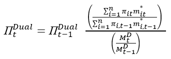
(2.11) where . Equation (2.11) shows that the growth rate of the Divisia index is a weighted average of the growth rate of the monetary components. The dual user cost index () to the Tornqvist-Theil Divisia index is defined by the following recursive formula:

(2.12)

Constructing Divisia Monetary Aggregates for Saudi Arabia

Data

The construction of the Divisia monetary aggregates requires data on quantities and prices of all components of monetary assets. The prices here stand for rental rates of the assets (user costs). Following the definition of monetary aggregates in Saudi Arabia, as defined by SAMA (Saudi Arabian Monetary Agency), the central bank, M1 and M2 are composed of the following:

M1 = currency in circulation + Demand deposit

M2 = M1 + Time and saving deposits (various maturities)

So, the data required for the construction of the Divisia index include the following:

Quantity of currency in circulation

Quantity of demand deposits

Quantity of time and saving deposits (various maturities)

The implicit rate of return on demand deposits

The rate of return on time and saving deposits (various maturities)

Treasury bill rates (various maturities)

Government bonds rates (various maturities)

The data sample is quarterly data ranging from (1993Q1) to (2006Q3). All data are obtained from the Saudi Arabian Monetary Agency (SAMA).

Calculating the implicit rate of return on demand deposits for Saudi Arabia

Usually, demand deposits yield no explicit interest rate under government regulations. However, most financial institutions pay implicit interest on demand deposits in the form of free or reduced-cost bank services, easier access to credit, and/or offer free gifts on promotional schemes. Laidler (1993) emphasizes that the assumption of zero interest on demand deposits is a false assumption and it would lead to variation in the quantity of money demanded. Some economists have suggested that such non-price competition has allowed depositories to elude the regulations that ban explicit interest on demand deposits.

According to Startz (1979), there are three hypotheses on the effectiveness of the Banking Acts of 1933 and 1935 prohibition of interest on demand deposits. The first one is the traditional hypothesis, which regards the prohibition to be fully effective. Second is the competitive hypothesis, which regards the prohibition to be completely ineffective. The third hypothesis is the modified competitive hypothesis, which regards the prohibition to be partially effective. Assuming that depositories face a perfectly competitive market, Klein (1974) derived an expression for the fully competitive implicit rate of return on demand deposits as follows:, (2.13) where r_D is the implicit interest rate on demand deposits, r_A is the interest rate on alternative assets, and c is the ratio of reserves to deposits. However, Startz (1979) emphasizes the use of the modified competitive hypothesis. Using functional cost analysis data, he argues that the implicit interest rate on demand deposits is well below the fully competitive Klein rate. Thus, the implicit rate of return on demand deposits is: , (2.14) where τ is the maximum reserve requirement on demand deposits, and α is a coefficient that lies in the interval [0.34-0.58]. The Startz (1979) approach is adopted to calculate the implicit rate of return on demand deposits for Saudi Arabia. The three-month Treasury bill rate was used as a proxy to the interest rate on alternative asset. α which is set to its maximum value of 0.58.

Calculating the Benchmark Rate of Return for Saudi Arabia

As illustrated in the Divisia theoretical section, the benchmark rate is necessary to calculate the user costs of monetary assets. According to Barnett and Spindt (1983), the benchmark rate is the highest rate among bond rates and all component assets at each period, this approach is called the “envelop” approach. In practice, benchmark rate should be defined in such a way that the user costs for monetary assets are positive. Anderson, Jones, and Nesmith (1997), constructed the benchmark rate during each period t as follows:

, (2.15) where r_it is the rate of return on monetary asset i at time t, r_BAA,t is the own rate of return on Moody’s seasoned BAA bonds at time t, and c is a small constant added to guarantee that the benchmark rate is strictly greater than the rate on any monetary asset.

To calculate the benchmark rate for Saudi Arabia we follow Anderson, Jones, and Nesmith (1997) approach. Thus, the benchmark rate for Saudi Arabia is

(2.16)where rdd is implicit rate of return on demand deposits, rtsd_i is a vector of the rates of return of time and saving deposits with different maturities ( one, three, six, and twelve month), rtbills_i is a vector of rates of return on Treasury Bills with different maturities (one-week, one-month, three-month, six-month, and twelve-month), and rbond_i is a vector of the rates of return on government bonds with different maturities (two, three, five, seven, and ten year).

A Comparison of Simple-sum and Divisia Monetary Aggregates for Saudi Araibia

Divisia aggregates have been computed for M1 and M2 categories defined by SAMA (Saudi Arabia Monetary Agency). Since the Divisia aggregates are an alternative to the conventional simple-sum aggregates, it will be instructive to compare them after normalizing so that both have the value of 100 at the same base period, 1993:1Q.

Table (2.1) illustrates the calculated Divisia aggregates along with their simple-sum counterpart. Furthermore, levels, annual growth rates, and income velocities are compared to contrast the behaviors of the Divisia aggregates with their simple-sum counterpart over the sample period.

M1 Graphical Analysis

Figure (2.1) plots the narrow money aggregates (M1). It shows a similar increasing trend for Divisia and simple-sum until early 1996, when they began to diverge but in the same direction. Overall, the Divisia and simple-sum M1 have a very small discrepancy between them. This could be explained by the high substitutability among M1 components, currency in circulation and demand deposits. Furthermore, simple-sum M1 reveals a higher level of liquidity compared to Divisia M1.

Figure (2.2) plots the annual growth rates for simple-sum and Divisia indices. Both Divisia and simple-sum M1 appear to share similar movements and the difference in the growth rate between them seems much smaller. Furthermore, both series are highly correlated, as observed in figure (2.2). However, the period between late 2001 and early 2002 reveals significant divergence between the Divisia and simple-sum M1 growth rates. This could be attributed to the huge inflow of the national financial investments from abroad to domestic banks in the aftermath of September 11 attacks. Since Divisia applies an implicit rate of return on demand deposits, less weight has been given to demand deposits than the case in simple-sum aggregate, which explains the lower rate of growth of Divisia M1. Table (2.2) shows the basic descriptive statistics of Divisia and simple-sum M1. In general, table (2.2) suggests that the growth rates of Divisia and simple-sum M1 do not differ much from each other, and their correlation coefficient is close to unity.

The conventional way to obtain income velocity is to divide income by the monetary aggregate. Nominal gross domestic product (GDP) is most commonly used as a proxy for the volume of transactions. However, for the case of Saudi Arabia, two different series are used as a proxy for the volume of transactions. The first one is the non-oil gross domestic production. The reason for using non-oil GDP instead of total GDP is due to the nature of the economy of Saudi Arabia. The Saudi economy is largely dependent on the production and exportation of oil which accounts for more than one-third of the total GDP. The oil revenues do not affect the transactions directly since all oil revenues accrue to the government. In other words, the oil sector value added is directly regulated by the government and it does not have a direct impact on private sector investment. However, the indirect impact on the private sector is through fiscal policy and mainly through government expenditures. Another reason for using the non-oil GDP is related to the fact that non-oil GDP is relatively more stable than GDP. This is due the instability of the oil market abroad. The second series is full income or total expenditure, obtained by adding expenditure on monetary services and expenditure on consumption goods from the representative’s budget constraint. This approach is also adopted to obtain income velocity of Divisia and simple-sum M2 also.

Income velocity of Divisia and simple-sum M1 using non-oil GDP are displayed in figure (2.3). In general, the discrepancy between the income velocity of Divisia and simple-sum M1 is very small and fairly stable until 2001. From 2001 to the end of the sample, the income velocities exhibit a downward trend and slightly expand discrepancy between the velocity of Divisia and simple-sum M1. This could again be attributed to the huge inflow of the national financial investments from abroad to domestic banks in the aftermath of September 11 events. Furthermore, in order to diversify the economy and stimulate foreign direct investment (FDI), economic reforms and deregulations of the financial system are introduced from 2000 and 2003. Data on FDI shows a significant upward trend since these reforms and deregulations were introduced. These vast inflows end up into different form of financial assets, hence expanding the monetary aggregates.

Figure (2.4) plots the income velocity of Divisia and simple-sum M1 using full income as a proxy for transactions. During the period 1993-2001, the velocity of Divisia M1 was more stable than the velocity of simple-sum M1, which was exhibiting a slight downward trend. By the end of 2001, both velocities show a persistent downward trend. This could be explained by the same reasons discussed earlier.

M2 Graphical Analysis

Figure (2.5) plots the broad money aggregates (M2). It shows a similar increasing trend for Divisia and simple-sum until early 1994, when they began to diverge but in the same direction. This divergence is due to the faster growth in simple-sum M2 compared to growth in Divisia M2. Overall, the Divisia M2 and simple-sum M2 aggregates have a larger discrepancy between them than those observed for Divisia M1 and simple-sum M1. This larger discrepancy could be attributed to the fact that broad money includes more financial products and instruments than narrow money. Thus, simple-sum M2 reveals a higher level of liquidity compared to Divisia M2.⁴

Figure (2.6) plots the annual growth rates for simple-sum M2 and Divisia M2 indices. In general, simple-sum M2 records higher growth rates than Divisia M2 except for the period from 2001 to 2002. Furthermore, both Divisia M2 and simple-sum M2 appear to share similar movements except for the period from late 2001 to early 2002. The period between late 2001 and early 2002 reveals significant divergence between the Divisia and simple-sum M2 growth rates. This could be attributed to the huge inflow of the national financial investments from abroad to domestic banks in the aftermath of September 11 events. Table (2.2) shows the basic descriptive statistics of Divisia (M1 and M2) and simple-sum (M1 and M2) aggregates. In general, table (2.2) suggests that the growth rates of Divisia M2 and simple-sum M2 are more volatile and less correlated than their counterparts Divisia M1 and simple-sum M1.

Income velocity of Divisia M2 and simple-sum M2 aggregates using non-oil GDP are displayed in figure (2.7). In general, the discrepancy between the income velocity of Divisia M2 and simple-sum M2 aggregates is larger than those exhibited by Divisa M1 and simple-sum M1. However, fairly stable income velocity for both Divisia M2 and simple-sum M2 are observed until 2001. From 2001 to the end of the sample, the income velocities exhibit a downward trend and slightly expand the discrepancy between the velocity of Divisia and simple-sum M1. This could, again, be attributed to the huge inflow of the national financial investments from abroad to domestic banks in the aftermath of September 11 events. Furthermore, in order to diversify the economy and stimulate foreign direct investment (FDI), economic reforms and deregulations of the financial system were introduced from 2000 and 2003. Data on FDI show a significant upward trend since these reforms and deregulations were introduced. These vast inflows end up into a different form of financial assets, hence expanding the monetary aggregates.

Figure (2.8) plots the income velocity of Divisia and simple-sum M2 using full income as a proxy for transactions. During the period 1993-2001, the velocity of Divisia M2 was more stable than the velocity of simple-sum M2, which was exhibiting a slight downward trend. By the end of 2001, both velocities show a persistent downward trend. This could be explained by the same reasons discussed earlier.

Appendix A

Note: SS. M1 and SS.M2 are simple-sum monetary aggregates M1 and M2,

Divisia M1 and Divisia M2 are Divisia monetary aggregates M1 and M2.

Table 2.2 Summary of Basic Statistics for Divisia and Simple-sum Aggregates

Notes:

1. Quarterly year-to-year change.
2. (DM1 and DM2) represents Divisia aggregates.
3. (SM1 and SM2) represents Simple-sum aggregates.

Chapter three

Literature review of the demand for money

Introduction

One of the most important issues in the theory and application of macroeconomic policy is the stability of the money demand function. This stability is a necessary condition for the accuracy of predicting the influence of money on real variables of the economy, as often emphasized by Milton Friedman. On the other hand, money demand holds a key position in macroeconomics in general and monetary economics in particular. Therefore, a stable money demand function is generally considered essential for the formulation and conduct of efficient monetary policy. Furthermore, considerable effort has been made in the empirical literature, for both industrialized and developing countries, to determine the factors that affect the long-run demand for money and assess the stability of the relationship between these factors and various monetary aggregates.⁵

By the mid- 1970s, however, the stability of the money demand function was questioned and the stable money demand function is no longer stable. This has been called the breakdown of the money demand function. The conventional M1 money demand function began to severely over predict the demand for money. Stephen Goldfeld labeled this phenomenon of instability in the demand for money function “the case of the missing money.”⁶

There are several opinions about what causes breakdown in the money demand function. However, there is general consensus among economists that financial liberalization and the advance of financial innovation in a number of developed, as well as some other developing; economies have significantly contributed to the breakdown in the demand for money.

The line that this work adopts deals with the measurement of money as the main cause for instability. All central banks around the world publish and adopt the use of the conventional Simple-Sum monetary aggregates as the measurement of money. Advocators of an aggregation theoretic approach to money demand argue that simple-sum measures are not consistent with microeconomic theory since the simple addition of components would be justified only in a case when all components are perfect substitutes for each other (see Barnett, 1980). Therefore, simple-sum monetary aggregates are likely to give an incorrect expression of the stock of money in the economy.

A Brief Overview of the Theory of Demand for Money

The fundamental theoretical literature which links the demand for money and modern macroeconomics will be surveyed in this section.⁷ Three essential features of money have provided macroeconomists the foundations for many theories of the demand for money. First is the use of money as the modern satisfactory medium of exchange and the customary units in which prices and debts are expressed. This feature led to transaction models which assume that the level of transactions is known and net inflows are dealt with by others as uncertain. Furthermore, the use of money as a medium of exchange boosts economic efficiency by reducing the opportunity cost of physically exchanging goods and services. Second, money functions as a store of value and serves the purpose of preserving purchasing power. Other assets can act as a store of value, but they either have an uncertain nominal return because of capital gains and losses, such as equity and bond, or they involve transaction costs in order to be converted into money. In other words, there is willingness to hold money and this is due to the convenience and liquidity of money. Third, money serves as a unit of account, which means that prices will all be quoted in terms of money.

There is widespread agreement among economists that the demand for money is primarily a demand for real balances.⁸ Money demand theories have evolved over time and the following will briefly shed light on the most influential developments.

The Quantity Theory

The quantity theory of money explains the role of money as a medium of exchange. In general, it is defined to hold that changes in the money supply induce proportional changes in the price level. This was presented by classical economists Fisher (1911) and Pigou (1917) under the classical equilibrium framework by two alternatives but equivalent expressions. They thought that money was neutral, with no consequences for real economic variables. Fisher analyzed the institutional details of payment mechanism in his work, which is known as Fisher’s Equation of Exchange. The concept of money holding by individuals was emphasized through the writings of Pigou, which is known as the Cambridge Approach “Cash Balance Approach.”

Fisher’s Equation of Exchange

Fisher’s equation gives special importance to the transaction demand for money, which is typically expressed by the following identity:

M^s V = P T (3.1)

Where Ms is the actual stock of money, V is velocity of transactions, P presents the price level, and T is the volume of transactions. The equation of exchange is an identity because it must be true that the quantity of money times how many times it is used to buy goods equals the amount of goods times their price.

To move towards the quantity theory of money, Fisher makes two key assumptions. First, Fisher viewed velocity as constant in the short run. This is because he felt that velocity is affected by institutions and technology that change slowly over time. Second, Fisher, like all classical economists, believed that flexible wages and prices guaranteed output, Y, to be at its full-employment level, so it was also constant in the short run.

Putting these two assumptions together, let’s look again at the equation of exchange:

MV = PY (3.2)

If both V and Y are constant, then changes in M must cause changes in P to preserve the equality between MV and PY. This is the quantity theory of money. A change in the money supply, M, results in an equal percentage change in the price level P.

The limitation of the Fisher approach is that velocity is not fixed; even in the short run it is unstable. It is, therefore, not independent of changes in money supply. In the real world, changes in money supply are not wholly absorbed by changes in price level. This approach also fails because empirical evidence does not often support the direct and proportional relationship between money supply and the price level. An example is the case of economic depression.

The Cambridge Approach

Cambridge economists such as Pigou (1917) and Marshall (1920) developed a different approach to the quantity theory of money. They recognized that money yields utility as it is accepted as a means of exchange. This approach is based on an individual’s behavior. Therefore, the determinants of money demand are different from those of Fisher’s quantity theory. The demand for money can be represented as follows:

M^d = k. PY or M^d / P = k Y (3.3)

Where k = 1/v

is the proportion of nominal income that an individual wants to hold as money. Incorporating the classical assumption of money market equilibrium, the Cambridge Approach leads to the quantity theory formulation. Under this approach, it is assumed that the real income y is at full employment level, and income velocity (V) is fixed. Therefore, the price level moves proportional to the quantity of money, “money is neutral.”

The Keynesian Approach

Keynes argued that velocity of money is unlikely to remain the same over time. He also emphasized the important role of interest rate in the money demand function and recognizes the function of money not only as a medium of exchange but also as a store of value. Therefore, both transaction and asset theories were considered in Keynes’ analysis. According to liquidity preference theory, “Keynes’ overall theory of the demand for money,” people hold money for three motives: transaction, precautionary, and speculative.

The transaction motive follows a similar emphasis as the quantity theory on money as medium of exchange. Keynes postulated that the transactions demand for money is a positive and stable relationship with the level of income. Because of the uncertainty about the future payments which individuals want or have to make, people hold additional money as a cushion against unexpected needs. The demand for the precautionary money balances are determined primarily by the level of transactions that individuals expect to make in the future, by the level of income, and slightly by the interest rate.

However, the most significant contribution of Keynes’ analysis of the demand for money to the theory of money demand is his speculative demand for money which emphasizes the store of value function of money and depends negatively on the interest rate. Keynes assumed that there exist only two types of financial asset, money and bonds. Money is a perfectly liquid financial asset, but earns no interest. Therefore, all non-interest-earning financial assets are regarded as money. Bonds include all interest-earning financial assets. They are less liquid, but earn interest returns. Therefore, the price individuals are willing to pay for bonds depends on the future rate of interest. In other words, people tend to hold money when they expect interest rates to rise (and therefore bond prices fall) and vice versa. Furthermore, Keynes introduced the idea of “liquidity trap” in which the interest elasticity of money demand can be infinite at low levels of interest rate. Keynes agreed with Fisher that the transaction demand for money was stable. However, he believed that the total demand for money could be dominated by unstable speculative individuals’ behaviors (Laidler, 1969) and, thus, be unstable.

Keynes assumption that individuals are to hold their liquid assets in the form of either money or bonds, but not both, is one of the major criticisms to Keynes’s analysis of the speculative demand for money. Tobin (1958) argued that people diversify their portfolio of assets to reduce risk.

By combining the three types of demands suggested by Keynes, we get the Keynesian liquidity preference function, which describes the total demand for money represented as:

(3.4)

with f₁ < 0 and f₂ > 0, where f_i denotes the partial derivative of f (.) with respect to it ith argument. That is, the demand for real money balances is negatively related to the nominal inte rest rate, R, and positively related to real income, Y.

Friedman’s Modern Quantity Theory

Unlike Keynes’ analysis of the demand for money, Friedman (1956) did not notice the motivation of people keeping money any more, instead of that, he assumes that money is a kind of wealth asset, and the reason why people choose different sorts of assets to save wealth is the main complication of money demand. Friedman integrated both an asset theory and a transaction theory of demand for money within the context of neoclassical microeconomic theory of consumer and producer behavior. He argued that demand for money should be treated in the same way as the demand for goods or services. That means viewing money as a durable good (or monetary assets as durable goods), which yields a flow of non-observable services.

According to Friedman (1956), wealth is categorized into human and non-human wealth. Human wealth is defined as the present discounted value of labor income, while the non-human wealth consists of the individual’s financial and physical assets. Therefore, the total wealth of an individual is the sum of five components: money, bonds, equity (common stocks), real assets, and human capital. Friedman emphasized using the ratio of human to non-human wealth as a proxy for the individual’s degree of uncertainty of wealth.

In Friedman’s view, the demand for money is a function of the wealth and the other assets that people hold and the expected return rate. However, since data on human and total wealth were not available, Friedman used permanent income as a proxy for total wealth. Furthermore, he argued that the permanent income of people is stable; it is the average expected of people’s long term revenue. During the period of expanding business, the provisional revenue is more than the permanent income. The average fluctuant extent of income is stable, and to permanent income, it is stable. In Friedman’s theory, permanent income is the main key of the function of money.

Therefore, according to Friedman, the demand for money can be expressed in terms of the following demand function of money for an individual wealth holder:

(3.5) where m^d is the demand for money in real terms, Y_p is the real permanent income, P is the price level, r_i is the yield in real terms on the ith asset, Π is rate of expected rate of inflation, and ω is the ratio of human to non-human wealth. In contrast to Keynes, Friedman concluded that the demand for money is insensitive and the permanent income is the determinant complication of demand for money; if the permanent income is stable, the demand for money will be stable. Thus, velocity is predictable.

The Baumol-Tobin Inventory Model

This model is based on the independent works of Baumol (1952) and Tobin (1956) and emphasizes the costs and benefits of holding money. It is argued, for example, that the benefit of holding money is convenience and the cost is the forgone interest by not holding interest-yielding assets. Furthermore, this approach viewed money as an inventory held for transactions purposes. Although higher yields could be earned by holding liquid financial assets other than money, the transactional costs of going between money and these assets justified holding such inventory.

The assumptions of the model are (a) the individual receives a known lump sum cash payment of T per period and spends it all, evenly, over the period; (b) there are only two assets, money and bonds, where bond holdings pay constant interest rate r per period and money pays zero interest; (c) a fixed brokerage fee b (transaction costs) may be incurred when the individual sells bonds to obtain cash in equal amounts K; (d) the key element in this inventory model is that all relevant information is known with certainty.

The total cost of making transactions is presented as, (3.6) where (Y/K) represents the number of withdrawals, b*Y/K is the sum of the brokerage fee, (K/2) is the average amount of real money holdings (= M / P), and R*K/2is the foregone interest if money is held instead of interest-yielding assets.

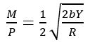
By minimizing the total transaction costs with respect to K, one arrives at the following optimal money demand, (3.7) Equation (3.7) shows that the optimal demand for money balances (M/P) depends on real income, transaction costs, and interest rate. This suggests that demand for money emerges from a trade-off between transactions costs and interest earnings.

Microfoundations and Aggregation Approach for Money Demand

Since the breakdown of the conventional money demand function in the mid-1970s, there has been a growing interest in developing firmer microfoundations for the demand for money. The focus shifted to providing a broader theory of demand for money based on simultaneous household and firm production and consumption decisions, rather than analyzing agents’ desired holdings of money as a separate problem.

Several theories have emphasized the role of microfoundations in analyzing the demand for money.⁹ For example, Lucas (1980) made seminal contributions in developing the cash-in-advance models to provide microfoundations for money and to extend the theoretical support for transactions demand for money. He incorporated the optimizing behavior of individuals, as discussed in Baumol (1952) and Tobin (1956), and the cash-in-advance constraint in a macroeconomic equilibrium setting to study the transactions demand for money. Also, McCallum and Goodfriend (1987) introduced the shopping-time model. They argue that the demand for money should be analyzed by taking explicitly into account the transactions facilitating services provided by money. In other words, they suggest that the use of money permits an individual to reduce the amount of time allocated to consumption. This frees up time available for labor and leisure activities, thereby boosting utility on the margin and generating implicit return.

Since the empirical methodology of this paper includes a model that is consistent with the principles of microeconomic and aggregation theory, an overview of this approach is presented in what follows. There are two branches of the microeconomic aggregation theory. The first one leads to the construction of index numbers and methods derived from economic theory. The second one leads to the construction of money demand functions in the framework of a system of equations which model the wealth holder’s allocation of total expenditures between money and non-money assets.

Diewert (1974) provides the theoretical basis for durable as well as non-durable goods in an intertemporal utility approach. Furthermore, the derivation of user cost of monetary assets by Barnett (1978) paved the way for formulation of a representative consumer’s decision problem over consumption goods, leisure, and services of monetary assets. Feenstra (1986) has shown that models which explicitly model the transaction services of money can be approximated as money in the utility function models.

Consider the representative household that is faced with the problem of allocating full income over consumption goods, leisure, and the services of monetary assets. The household must choose a vector of commodity consumption quantities (c), a quantity of leisure (), and a vector of the services of monetary assets (x) to maximize U (c, l, x) subject to q‘c + π‘x + ωL = y (3.8)

where y is full income ( i.e., income reflecting expenditures on consumption goods as well as on time and services); q is a vector of the prices of c; π is a vector of monetary asset user costs (or rental prices) as defined in the Divisia chapter; ω is the shadow price of leisure (see Barnett, 1981b). Following Robert Strotz (1957, 1959) and William Gorman (1959), the representative household is assumed to solve a two-stage decision process. In the first stage, expenditure is budgeted among broad categories (consumption goods, leisure, and monetary services) based on price indexes of these categories. In the second stage, the budgeted expenditure on each category is allocated over its components.¹⁰

Furthermore, the assumption of homothetic weak separability of the representative consumer’s utility function is essential to ensure that the two-stage budgeting procedure is an accurate description of consumer behavior. In other words, without weak separability a utility function in money alone does not even exist. Thus, it must be possible have the utility function written as u = U (c, l, f(x)) (3.9) in which f is the monetary subutility function. A necessary and sufficient condition for weak separability is that the marginal rate of substitution between any two monetary assets is independence of the value c and l¹¹. That is

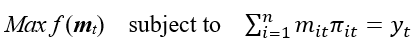
for i ≠ j (3.10) where ζ is any component of {c, l }. Once the separability subset of assets is established, then we can focus on the demand for services of monetary assets alone. This can be seen by solving the following neoclassical consumer problem, max f (x) subject to π‘ x = y_m (3.11) where y_m is the expenditure on the services of monetary assets (determined in the first stage of the two level optimization problem) and π is a vector of monetary asset user costs as defined above. To derive the money demand function, we set the Lagrangean for the consumer’s problem as follows, L = f (x) – λ (y_m – π‘ x)

The first order conditions are, f_i (x) = λ π_i y_m = π‘ x where f_i (x) is the partial derivative with respect to x_i.

Solving the system of simultaneous equations derived from the first order conditions yields the demand system for monetary assets, x_i^* = (π, y_m) which express the dependence of the demand for monetary assets on user costs and income.

Literature Review of Money Demand in Saudi Arabia

In Saudi Arabia, like other countries, considerable effort has been made in estimating money demand functions. For example, Darrat (1984), Nagadi (1985), Ghamdi (1989), Al-Bassam (1990), Metwally and Rahman (1990), Alkswani and al-Towaijari (1999), Al-Badi (2002), and Harb (2003), etc., have estimated money demand functions by using alternative specifications. All of these studies have also examined the stability of their estimated money demand functions. Generally, the M1 and M2 functions are found to be stable, and the effect of the interest rate on the money demand functions is low and statistically insignificant.

Alkswani and al-Towaijari (1999), investigated the determinants of the money demand function for Saudi Arabia for the period from 1977 to 1997 using quarterly data. Employing the Engle and Granger cointegration approach, they concluded that the relationship between real money M1, the real income, the interest rate, the inflation rate, and the exchange rate is significantly different from zero. However, the effect of the interest rate on the demand for money is still very low compared to the average in other countries, which is explained by the social and religious rationales of the people of Saudi Arabia.

Using annual data that cover the period from 1969 to 1999, Al-Badi (2002) investigated the demand for money in Saudi Arabia. He used the ARDL approach to determine the relationship between money demand (M1, M2, and M3) and its determinants (Income, Financial Development, Foreign Interest Rate, Expected Rate of Inflation, and Real Exchange Rate). The results indicated that money demand is determined by income and the degree of financial development only.

Harb (2003) estimated the money demand function for the GCC (the Gulf Cooperation Council) countries using heterogeneous panel cointegration tests. He employed the use of Fully Modified Least Squares (FMOLS) to estimate the idiosyncratic elasticities of money demand function. The results showed a strong evidence of cointegration amongst the estimated variables. Although the estimated elasticities have the expected signs, only in the case of the scale variable are they significantly different than zero. However, Harb (2003) found a significant negative semi-elasticity of money demand with respect to interest rate when allowing for heterogeneity among GCC countries.

Chapter four

Hypothesized models and methodology

Two alternative approaches will be employed to estimate the money demand function for Saudi Arabia using two different measures of monetary aggregates (Divisia and Simple-Sum monetary aggregates). The first approach is the conventional way, which is based on empirical literature where non-oil GDP is used as a measure for income. The reason for using non-oil GDP instead of using total GDP will be discussed below. The second approach is the consumer demand theory approach to money demand. This approach emphasizes the use of microeconomic and aggregation theory and deals with monetary assets as durable goods which are directly entered as arguments in the household utility function. The Johansen cointegration technique and error correction models will be employed to examine the long-run and short-run concepts of the demand for money in Saudi Arabia in both approaches.

Hypothesized Models

The Conventional Approach for Money Demand Function

From the literature reviewed, there is generally a consensus among money demand theories that the main determinants of the quantity of money demanded are the scale variable, which can be real income, wealth, or permanent income and opportunity cost variables (Goldfeld & Sichel, 1990). Therefore, the money demand relationship can be written as the following M_t/P_t = Ф (R_t, Y_t) (4.1) where

M_t = demand for nominal money balances;

P_t = the price level;

Y_t = scale variable (income, wealth, or expenditure, in real terms); and

R_t = vector of opportunity cost of holding money.

The function Ф is assumed to be increasing in Y_t , decreasing in those elements of R_t representing rates of return on alternative assets, and increasing in rates of return associated with assets included in M_t.

Scale variable

Income, which is defined as non-oil GDP, is the choice of the scale variable because of data limitation on wealth. The reason that income is measured in term of non-oil GDP rather than in term of the GDP is the nature of the Saudi Arabian economy. The Saudi economy is largely dependent on the production and exportation of oil, which accounts for more than one-third of the total GDP. The oil revenues do not affect the private sector’s demand for money, since all oil revenues directly accrue to the government. In other words, the oil sector value added is directly regulated by the government and does not have a direct impact on private sector investment. However, the indirect impact on the private sector is through fiscal policy and mainly through government expenditures. Another reason for using the non-oil GDP is related to the fact that the non-oil GDP is relatively more stable than the GDP. This is due to the instability of the oil market abroad. Therefore, using non-oil GDP as a measure for the budget constraint is proposed.

Opportunity cost variable

The opportunity cost of holding money is the second independent variable that determines the money demand function. There is substantial empirical evidence that the demand for money is negatively related to the rate of interest in almost all financially developed economies as well as many developing economies. However, the literature of money demand in Saudi Arabia showed an insignificant role for the rate of interest. There are three reasons that may contribute to this insignificance of the interest rate. First is the presence of the government-sponsored institutions that provide low-cost loans (Al-jasser & Banafe, 1999).¹² Second, most developing countries, including Saudi Arabia, lack the financial depth that could provide a wide range of alternative financial assets other than time and savings deposits. Third, Islamic law prohibits any kind of transactions that explicitly involve an interest rate.

On the other hand, the literature on money demand in Saudi Arabia used the Eurodollar rate (the foreign interest rate) as a proxy for the opportunity cost of holding money. The reason for doing so is due to the openness of Saudi Arabia’s economy. Therefore, the money lenders tend to lend overseas at the Eurodollar interest rate (Metwally & Abdelrahman, 1990). However, this study will investigate the significance of both the domestic and foreign interest rates as an opportunity cost variable for holding money in simple-sum models. On the other hand, the significance of the dual price, which represents the opportunity cost variable, for Divisia indices will be investigated in Divisia models.

Another variable that is used as a proxy for the opportunity cost of holding money is the expected rate of inflation. Expected inflation is added since holding wealth and durable goods may be the most appropriate alternative to holding money. However, since inflation was near zero, and sometimes negative, during the study sample period, this variable will not be considered in the analysis.

The last variable that will be added in the specification of money demand function is the real exchange rate, to serve as a proxy for the external factors and capturing the openness of Saudi economy. Given the fact that the Saudi riyal is pegged to the U.S dollar, any fluctuation in the value of the U.S dollar relative to other international currencies will affect the value of the riyal and, hence, the demand for money in Saudi Arabia. The SDRs (Special Draw Rights) of the International Monetary Fund is used as a proxy for the exchange rate variable since it represents an average of the exchange rate versus a set of other currencies. The definition of the exchange rate is the number of Saudi riyal per one unit of SDR. Therefore, an appreciation of the Saudi riyal is seen as a decrease in the exchange rate. Because no series on expected exchange rate is available, the actual series were used as a proxy.

Therefore, the proposed long-run money demand function for Saudi Arabia specified in a log-linear form, with the exception of domestic interest rate, real exchange rate, and foreign interest rate, is:

(4.2) where M represent Divisia (M1, M2) or Simple -Sum (M1, M2) monetary aggregates, Y_non is the transaction volume that is approximated by the non-oil gross domestic product, r is the domestic interest rate when M is considered as either simple sum M1 or M2 monetary aggregates and is the dual price user cost when M is considered as either Divisia M1or M2 monetary aggregates, REX is the real exchange rate, r^f is foreign interest rates (Eurodollar rate), and ε_t is the error term.

Following macroeconomic theory, a positive sign is expected for income coefficient, while the opportunity cost coefficients, domestic and foreign interest rates, are expected to be negative. As for real exchange rate coefficient, it could be negative or positive. If the increase, or depreciation, in exchange rate is perceived as an increase in wealth, then the demand for domestic money increases, yielding a positive coefficient. However, if the increase induces an expectation of further depreciation of the domestic currency, the public may hold less domestic currency and more foreign currency. In this case, the expected sign of real exchange coefficient is negative.

The Consumer Demand Theory Approach for Money Demand Function

This approach emphasizes the microeconomic theory and implies microeconomic aggregation and index number theory. Furthermore, it insists on having an internally consistent and methodologically coherent research. Based on this approach, the conventional set of the money demand function, which led to the breakdown in money demand function, and the variables used in applying it have no connection in a valid manner with economic theory. Barnett (1997) argues that including real income and interest rate as explanatory variables in money demand functions are not consistent with demand theory. Since the Divisia index is derived from a utility maximization framework, the demand for Divisia money should be modeled according to demand theory as the second stage of the budget allocation where the agent allocates his expenditure among consumption and monetary services. Therefore, defining the correct variables that must be included in the money demand function is presented here.

The Opportunity cost variable

Using an interest rate as the opportunity cost of money in demand for money equations is a common practice. According to index number theory, every quantity index has a dual price index, and vice versa. For the Divisia index, the price dual to the Divisia index, derived by Barnett (1978, 1980a), is the correct price, opportunity cost variable, for monetary services. In the case of simple-sum index, since the simple-sum monetary aggregate is a quantity index, then its dual price index must be considered instead of the interest rate.

Simple-sum quantity index assumes equal coefficients, which is a special case of the linear index. Therefore, the price dual to the linear quantity is the Leontief price index.¹³ The perfect substitutability implied among components of monetary assets induces corner solutions. This means that only the lowest-priced component will be held. Therefore, the correct price to associate with the Simple-Sum monetary aggregate is , (4.3) where n is the number of monetary assets included in the aggregate, and π_it is the user cost in terms of forgone interest for the monetary assets i which is defined as follows (4.4) where r_it is rate of return on monetary asset i, and R_t is the rate of return on the benchmark asset.¹⁴

The Income variable

Gross National Product (GNP) or Gross Domestic Product (GDP) are the most commonly used variables as a measure for income variable. However, GDP does not correspond to the representative agent’s income as it appears in the budget constraint. In other words, the right-hand side of the representative agent’s budget constraint does not express GDP. Furthermore, investment which is considered as one of the components of the GDP, does not appear in the representative agent’s budget constraint. On the other hand, GDP does not include expenditure on monetary services, which is considered as part of the household’s expenditure.

Barnett (1997) explained this in the following terms: “To make sense, a demand function that has income on its right hand side must imply the existence of a constraint containing that income variable on the right hand side of the constraint” (p. 10).

This is defined as: (4.5) where m_it is the component monetary asset having user cost π_it , is expenditure on monetary services, c_it is the component consumption having price p_it, is expenditure on consumption goods, and y_t is full income or total expenditure variable.

Therefore, the proposed long-run money demand function for Saudi Arabia, specified in a log-linear form, with the exception of the opportunity cost variable, is: (4.6)

where M represent Divisia (M1, M2) or Simple-Sum (M1, M2) monetary aggregates, P is the price level, Y is real expenditure on monetary services plus real expenditure in consumption (full income) obtained from the representative’s budget constraint, π is the price dual (the Leontief price index) when M is considered as either Simple-Sum M1 or M2 monetary aggregates and is the Divisia dual price user cost when M is considered as either Divisia M1or M2 monetary aggregates, and ε_t is the error term. The theory expects α₁ to have a positive sign and α₂ to have a negative sign. This reflects the positive and negative relation of income and opportunity cost variables, respectively, to the quantity of real balance demanded.

Methodology

Two different techniques are conducted to estimate the money demand function for Saudi Arabia. The first method is the widely used cointegration and error correction technique in the framework of the linear multivariate vector autoregressive (VAR). The second method is the Artificial Neural Network (ANN) technique that attracted much attention as a relatively new method for estimating and forecasting in economics and finance. Artificial Neural Network (ANN) models are non-linear statistical models, no linearity limitations, based on the neural structure of the brain. These two techniques will be applied to the conventional and consumer demand theory approaches of estimating the money demand function using both Divisia aggregates data and Simple-Sum aggregates data as measures of monetary aggregates.

The Linear Technique (Cointegration and Error-correction)

This work will utilize different time-series techniques to investigate the existence of the long-run relationship between the alternative monetary aggregates and their determinants. A testing procedure suggested by Johansen (1988) and Johansen–Juselius (1990) will be conducted to examine possible cointegration among the variables. Vector error correction models (VECM), and innovation accounting, which include impulse response functions (IRF) and variance decomposition (VDC), are other methods used to analyze the short-run dynamics of the variables.

a.Unit Root Tests

The stationary of time series can have a strong influence on the behavior and properties of the data. Four unit root tests are used in this study to analyze the properties of the time series. The first two are the Augmented Dickey-Fuller (ADF) (Dickey & Fuller, 1979; 1981, Said & Dickey, 1984) and Phillips-Perron (PP) (Phillips, 1987; Perron, 1988) statistics are the most frequently used test for unit roots. An Augmented Dickey-Fuller (ADF) test can be specified as:

Where Yt is a random variable possibly with non zero mean, μ is a constant, t time trend and ε is the error term with mean zero and a constant variance. The null hypothesis of a unit root (τ= 1) is tested against the alternative of stationarity. However, the estimated τ does not have a standard t-distribution and hence the critical values provided by MacKinnon (1991, 1996) have to be used. The Zt statistic of Phillips and Perron (1987, 1988) is a modification of the Dickey-Fuller t statistic which allows for autocorrelation and conditional heteroscedasticity in the error term of the Dickey-Fuller regression. This is based on the estimation of the following equations:whereYt is the variables under consideration, T is the number of observations, μ and β are non-zero mean and linear trend terms, respectively.

The third unit root test is the Dickey-Fuller Generalised Least Squares (DF-GLS)¹⁵. The DF-GLS is a more powerful test than the Dickey-Fuller test. It is a modification to the ADF regression in which data are detrended before the unit root test is conducted. This detrending is done by taking the explanatory variables out of the data. The following equation is then estimated to test for a unit root in the variable:

where Δ is the difference operator,is the generalised least squares detrended value of the variable, α and ψ_j are coefficients to be estimated and εt is the independently and identically distributed error term. As in the case of the ADF test, a test for a unit root of the variable y involves examination of whether the coefficient of the AR(1) term, in this case α , in equation (#) is zero against the alternative hypothesis. In making inferences, the critical values tabulated in Elliott, Rothenberg and Stock (1996) are used in this study.

The fourth test is the Elliott, Rothenberg and Stock (ERS) Point Optimal Test. The ERS point optimal test has been found to dominate other commonly used unit root tests, when a time series has an unknown mean or a linear trend. This test is based on the following quasi-differencing regression:where d(yt(a) and d(zt(a) are quasi-differenced data for Yt and Zt respectively and ηt is the error that is independently and identically distributed. Details on computing quasi differences are given in Elliott, Rothenberg and Stock (1996). In equation (#),yt is the variable whose time series properties are tested,zt may contain a constant only or both constant and time trend and δ (a) is the coefficient to be estimated. ERS recommend the use of α for a in equation (#).α is computed aswhen zt contains a constant andwhen zt contains a constant and time trend. α=1 and α =a are respectively the null and alternative hypotheses tested In the ERS point optimal test. The relevant test statistic (PT) to test the null hypothesis is:where SSR is the sum of squared residuals from equation (#) and f0 is an estimator for the residual at frequency zero. In making inferences, the test statistic calculated is compared with the simulation based critical values of ERS.

b.Cointegration Test

When working with economic time series, one often encounters nonstationary variables. These variables tend to grow over time and do not have a stationary mean. However, a group of nonstationary variables may jointly be converted into stationary by linear combination. Such variables are said to be cointegrated. Therefore, a useful preliminary step to performing any regression analysis is to uncover the properties and characteristics of the actual data involved. Such an analysis of the individual time series variables is important because the properties of the individual series have to be taken into account in modeling the data generation process of a system of potentially related variables (Lutkepohl & Kratzig, 2004). Some of the characteristics may have an impact on the statistical inference used in modeling and analyzing the underlying economic system. The first step is the notion of whether a series is stationary or not. Stationarity of the series is a desirable property for an estimated model. A series is considered stationary if it has a constant mean, constant covariance, and constant autocovariances for each given lag (Brooks, 2002; Lutkepohl & Kratzig, 2004).

The concept of cointegration was introduced and developed by Granger (1981) and Engle and Granger (1987). There are two important ways for cointegration analysis: single equation methods and system methods. Engle and Granger’s (1987) approach is a method based on assessing whether single equation estimates of the equilibrium errors appears to be stationary. This technique is a two-stage residual-based procedure.

Although the Engle and Granger technique is easily implemented, it suffers from several important defects. For instance, if more than two variables appear in a cointegration relationship, then running the usual cointegrating regression will not yield consistent estimates of any of these cointegrating parameters (Kennedy, 2003). Another defect of the Engle-Granger procedure is that it relies on a two-stage estimator. Hence, any error introduced by a researcher in stage one is carried into stage two (Enders, 2004). The suitability of the Engle and Granger approach is for the bivariate case, which can have at most one cointegration vector (Apostolo, 2001).

To overcome the limitations associated with the Engle-Granger technique, a researcher should consider system methods instead of single equation methods. Johansen (1988) and Johansen and Juselius (1990) proposed a procedure for estimating cointegration relationships in a system of equations framework. The Johansen technique provided maximum-likelihood estimates for testing more than one cointegrating vector in a set of time series. This technique is set to account for long-run properties as well as short-run dynamics, in the framework of multivariate vector autoregressive models. Cointegration tests in this paper are conducted by means of the method developed by Johansen-Juselius (1990) since this particular method is claimed to be superior to the single-equation Engle and Granger approach.

a.1 Johansen-Juselius technique

The Johansen-Juselius technique is a maximum-likelihood procedure for testing for cointegration in a finite-order Gaussian vector autoregression (VAR):(4.7)

Where Y_t is a p x 1 vector of the variables that are included in the estimated system, π_i is a p x p matrix of coefficients on the i^th lag of Y_t, K is the maximum lag length, µ is a vector of constants, D_t is a vector of exogenous variables, and ε_t is a vector of error terms such that ε_i ,……, ε_T are i.i.d N(0,Λ).

To explicitly distinguish between the short-run dynamics and the long-run static disequilibrium response, equation (7) is rewritten in vector error-correction form as: (4.8)

Whereand

The main focus of the Johansen-Juselius technique is on the parameter matrix Π (pxp), which contains information about the long-run relationship between the variables in Y_t . The rank of the matrix Π is the key feature to note. If matrix Π has either full rank, rank (Π) = P, or has rank (Π) = 0, then the cointegrating relationship does not exist. However, in the case when 0 < rank (Π) = r < p, there are r cointegrating relations among the elements of Y_t. Matrix Π can be decomposed as:Π = α β

Where β is (r x p) matrix of cointegrating vectors and α is (p x r) matrix of the speed of adjustments. So, the β vector stands for the estimation of the long-run cointegrating relationships between the variables in question. The α parameters measure the speed at which the variables adjust to restore a long-run equilibrium.

The number of distinct cointegrating vectors can be obtained by checking the significance of the characteristic roots of matrix Π (Enders 2004). Johansen proposed two likelihood ratio test statistics for testing the hypothesis of r cointegrating vectors. The first one is the trace test statistic. It tests the null hypothesis that there are, at most, r cointegrating vectors against a general alternative by calculating the following test statistic:(4.9) where λi(i = 1,…….,p) are the estimated values of eigenvalues obtained from the estimated Π matrix, T is the number of observations, and p is the number of endogenous variables in the system.

The second statistic is the maximum eigenvalue test. This statistic tests the null hypothesis that the number of cointegrating vectors is r against the alternative of (r + 1) cointegrating vectors. This is given as: (4.10) where λi are eigenvalues and they are calculated based on the two residual matrices obtained from the regression ofandonwhere i = (1,……, k-1).

A lag length must be determined for the VAR model in order to implement the Johansen procedure. Specifying the appropriate lag length of the VAR system makes the residuals uncorrelated. The literature describes several methods that have been used to determine the VAR order, such as the Sequential Modified Likelihood Ratio (LR), the Final Prediction Error (FPE), Akaike Information Criterion (AIC), Schwarz Information Criterion (SC) and Hannan-Quinn Information Criterion (HQ). Although these methods may produce conflicting VAR order selections, the aim is to use the one that produces the best possible results that conform to economic theory (Seddighi et al., 2000, p. 309).

The Johansen-Juselius technique provides a framework in which the alternative hypothesis about elements of α and β matrices can be tested. For instance, the null hypothesis that the long-run income elasticity of money demand is unitary and/or interest elasticity is zero can be tested. Also the hypothesis of the long-run exclusion of any variable in our model from the cointegration space can be tested. To test such hypotheses, a model incorporating the test restriction is compared with an unrestricted model. The likelihood ratio test statistics are given as:(4.11) and has a X² distribution with (p – r) degrees of freedom.

b. Vector Error Correction Model (VECM)

Vector Autoregressive (VAR) is no longer optimal when the variables that have unit roots are cointegrated. Engle and Granger (1987) showed that it is appropriate to estimate Vector Error correction models (VECM) instead of VAR in the case where cointegrated variables exist. A VEC model is a restricted VAR that has cointegration restrictions built into the specification. Therefore, VEC models are designed for use with nonstationary series that are cointegrated (Hamilton, 1994).

The VECM approach has the advantage of jointly estimating the long- and short-run components of the demand for money, thus facilitating the task of ensuring that short-run specifications are associated with long-run components consistent with established economic theory. The Granger representation theorem states that if two or more variables are cointegrated, that is, if there is a long-run relationship between them, then the short-run dynamic can be described by an error-correction model.¹⁶ Thus, the VEC models can be explained as, if an economy is not in equilibrium, then at least one of the variables has to correct this disequilibrium by adjusting accordingly to get the economy back to equilibrium (Sweidan, 2004). The speed of adjustment to equilibrium is measured by the vector error correction model. Arize and Shwiff (1993) summarize the desirable properties of the ECM as follows:

First, it [ECM] avoids the possibility of spurious correlation among strongly trended variables. Second, the long-run relationships that may be expressing the data in differences to achieve stationarity are captured by including the lagged levels of the variables on the right-hand side. Third, the specification attempts to distinguish between short-run (first-differences) and long-run (lagged-levels) effects. Finally, it provides a more general lag structure, which does not impose too specific a shape on the model (Hendry, 1979).

In VECM, the short-run dynamic adjustments of all endogenous variables are explicitly modeled as linear function of their own lags and lagged values of the remaining variables, subject to the coefficient restrictions imposed by the long-run cointegrating relation expressed in Equation (8). Therefore, instead of having only one error correction, the VECM consists of p error-correction representations, (Kennedy, 2003). The VECM representation is: 4.12) whereandare vector autoregressive (VAR) components in first differences and error correction components in level, respectively. Y_t is px1 vector of variables that are integrated of the same order. μ is a p x 1 vector of constants. k is the lag structure, while ε_t is p x 1 stationary random process with zero mean and constant variance (white noise error term). Г_i is a p x p matrix that represents short-run adjustments among variables. П is decomposed into αβ as explained in the cointegration section. Where β is an r x p matrix of cointegrating vectors and α is p x r matrix of the speed of adjustments.

c. Innovation Accounting Analysis

Two methods are implemented to investigate and analyze the dynamic interaction in our findings. The first one is the Impulse Response Function (IRF), and the second one is Variance Decomposition (VDC). Sims (1980) introduced the method of impulse response function to analyze the direction and the dynamic interaction among variables in the VAR system. The Impulse Response Functions trace out the time paths of the effects of one time shock or error in one variable on some or all of the other variables in the system. Thus, The IRF provides the means to investigate dynamic behaviors of certain variables caused by unexpected shocks in one of the variables. IRF can be used to examine the interaction between the variables sequences in the moving average representation. Usually IRF can be obtained from a moving average representation of the VAR model: Y_t = A₁ Y_t-1 + A₂ Y_t-2 + ……..+A_p Y_t-p + ε_t (4.13) Also the MA representation can be written as: (4.14) where φ is the coefficients of IRFs that are used to generate the effects of the shocks (ε_t-i) on the whole time path of thesequences. Since unstable, integrated, or cointegrated VAR (P) process does not possess valid VMA representation, the estimated VECM, instead of the VAR, is transformed into an infinite order VMA model in this study.

Variance Decomposition (VDC) is the second tool that is used to characterize the dynamic behavior of the VAR or VEC models. This tool reflects the proportion of forecast error variance of a variable which is explained by its own innovation, as opposed to that proportion attributable to innovations in other variables at different horizons. The variables are interdependent or jointly determined if the change associated with one variable explains some of the forecast error variance of the other variables.

Non-linear Technique (Neural Network Model)

Artificial Neural Network models (ANN) have been used for a wide variety of applications, including financial forecasting, macroeconomic, credit scoring, bond rating, and business failure prediction, where statistical methods are traditionally employed. Inspired from the biological neural network, ANN models are a class of input-output models developed using software that attempts to mimic the human brain’s ability to classify patterns or to make predictions or decisions based on past experience (Gately, 1996).

The origin of neural networks dates back to the 1940s. McCulloch and Pitts (1943) and Hebb (1949) investigated the ability of networks of simple computing devices to model neurological activity and learning within these networks, respectively. Minsky (1954) developed the computing platform on which current ANN models are processed. Later, the work of Rosenblatt (1962) focused on computational ability in perceptrons, or single-layer feed-forward networks. Rumelhart, Hinton, and Williams (1986) further enhanced the analysis using neural networks by introducing the generalized delta rule for learning by back-propagation, which is today the most commonly used training algorithm for multi-layer networks.

The main principles of the ANN models are massive parallelism, nonlinear neural unit response to neural unit input, processing in multiple layers, and dynamic feedback among units. In econometric terms, ANN models are a particular class of nonlinear time series models, where “learning” corresponds to the statistical estimation of model parameters. The ability of ANN models to learn by themselves makes them extremely adaptive to rules and relationships that are difficult to specify. Therefore, they have the ability to approximate whatever functional form that best characterizes the data.

Most of the ANN models consist of a vector of inputs, hidden layer, and output layer, connected by weights. One of the most popular types of ANN models is BPN (Back Propagation Network). The BPN model, a feed-forward model, will be used to compare the explanatory power of both Divisia and Simple-Sum monetary aggregates in estimating the money demand function using Saudi Arabian data.

a. The Back Propagation Network (BPN) and the Training Rule

The Back Propagation Network (BPN) is currently the most general-purpose and commonly used neural network paradigm (Swingler, 1996). BPN learns to generate a mapping from the input pattern space by minimizing the error between the output produced by the network and the desired output across a set of input vectors.

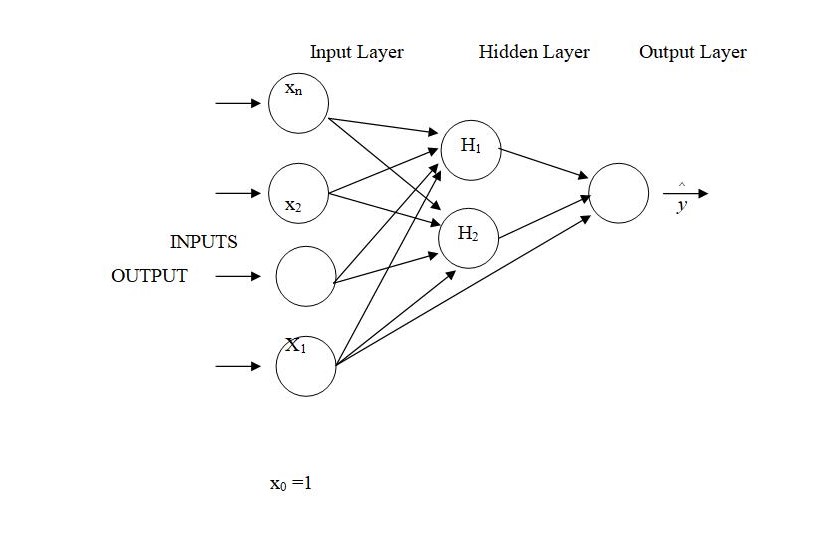
Figure 4.1 displays the architecture of a feed-forward neural network model that consists of three layers: an input layer, hidden layer, and output layer. In addition, a constant input term could be added, which for convenience may be taken as 1. The input layer X can be presented by a vector X = (x₀=1,x₁,…..,x_n), the hidden layer M consists of a vector of m = ( m₁,…..,m_k), and the is the produced output. The network is fully connected. That is, all neurons in each layer receive connections from all neurons (units) in each preceding layer. These connections are weights and there are two set of weights (β, γ), β for the connection between the input layer and the hidden layer and γ for hidden layer connection to output layer. It is a feed-forward network where input travels through the network to produce an output.

After the inputs and the output are read into the model, each input into a neuron is assigned a weight (coefficient) representing the relative importance of the input in the network. Then the values for the input variables are multiplied by their corresponding weight. Thus, the signal going into each of the hidden neurons is the weighted sum of the inputs:

net_j = Σ_i β_ij x_i (4.15)

j = 1, 2,…, k i = 0,1,….,n where β_ij is the connection weight from ith input unit to the jth hidden layer unit.

Then the weighted sums are converted to output through the training algorithm or activation function, which limits the sum to a specified range that is passed to a connected neuron in the hidden layer (Haykin 1999).

m_j = F (Σ_i β_ij x_i ) (4.16) where F is the activation function. These activation functions are mostly non-linear functions. If they were linear, then the output would simply be a proportional value of the input, and most of the ANN robustness would be lost (Fausett 1994). A commonly used function is the nonlinear sigmoid or logistic transfer function, which gives values between 0 and 1, and defined as

(4.17) where the value of α determines the steepness of the function.

In the same way, the output unit receives the weight sums (outputs) of the hidden layer units as their inputs and applies the same function as in the hidden layer units. The output of the output layer unit is defined as: = G (Σ_j γ_j m_j), (4.18)

j = 0,1,……,k where G is the transfer function, γ_j is the weight of the connection from the jth hidden layer unit to the output unit, and j = 0 indexes a bias or constant term with m₀ =1.

This output is compared to the corresponding target output and an error is produced. The back propagation learning rule method is applied to minimize the sum of the squared error of the system. That is, the network adjusts the weights (or coefficients) in the direction to reduce the error. Then another output will be generated and a new error would be calculated and so on. The network would stop when a certain specified error is reached. The back propagation learning rule method is a recursive gradient descent method that minimizes the sum of the squared error of the network. In other words, the network weights are chosen to minimize the error function,

(4.19) where N is the sample size, y_t is targeted (or observed) output value and Yt is the calculated output value.

The generalized delta rule is a common learning rule used in the Back propagation network model, which updates the weight for each unit as follows:

(4.20) where w is the weight for either the connection from the ith input unit to the jth hidden layer unit or the weight from the jth hidden layer unit to the output unit, η is the learning rate (typically less than 1), and∇ is the gradient vector associated with either the weight from the ith input unit to the jth hidden layer unit or the weight from the jth hidden layer unit to the output unit. A chain rule is used to calculate the gradient vector on a layer-by-layer basis.

A gradient descent procedure searches for a minimal error on the error surface. The error surface is multi-dimensional and may contain many local minima. Therefore, it is possible for the gradient descent learning algorithm to get trapped in a local minimum instead of a global minimum. There are several ways to keep the network from getting stuck in local minima. One of the ways is to restart the program with different weights and adjust the learning rate. Also, a genetic algorithm could be used, as suggested by Dorsey and Mayer (1995). Finally, a momentum term could be added to the weight update rule. Momentum terms are used to keep the weights changing in the established direction. That is,

(4.21) where, η is the learning rate, which affects how fast the network corrects its estimates, andis a momentum term added to avoid getting stuck in local minima and to accelerate the training. The above procedures are repeated for all patterns until the convergence is achieved.

Chapter five

Empirical analysis

This section focuses on empirical studies and analyses that illustrate the variation between the two approaches for estimating the money demand function discussed in the previous sections using two alternative monetary aggregates (Simple- Sum aggregates and Divisia aggregates). Two alternative techniques, linear (Cointegration and Error-correction) and non-linear (Back Propagation Neural Network), are used in the estimation of the demand for real money balances in the long and in the short run. Before estimating and analyzing the long-run and short-run money demand functions, the data and their sources are presented. The rest of the section is divided into two parts. The results from cointegration and error-correction technique are presented and analyzed in the first part. The second part presents and analyzes the results from the Neural Network technique. The conclusion is drawn at the end.

Data

The time series data used for estimating the money demand function in this study consist of quarterly observations covering the period form 1993:01 through 2006:03 for Saudi Arabia. The variables considered are money supply, narrow and broad definitions, gross domestic product (GDP), non-oil gross domestic product (NOGDP), household private expenditure, the Eurodollar rate, consumer price index (CPI), and exchange rate. Since only annual data are available for GDP and household consumption expenditure, the quarterly data on GDP and household consumption expenditure were interpolated from annual data using the Quadratic match sum interpolation method as provided by Eviews software. Quarterly data on the oil production, which consists of around 40 percent of the country’s gross domestic product (GDP), are used as a proxy for interpolating the GDP.

The Eurodollar rate (foreign interest rate) is used as a measure of opportunity cost in Saudi Arabia as explained in the model specification section. The IMF’s composite currency unit SDR (Special Draw Rights) is used as a proxy for the exchange rate variable. The definition of the exchange rate is the number of Saudi Riyal per one unit of SDR. The money supply data is represented by the simple-sum data, M1 and M2, and the constructed Divisia M1 and M2 data. The construction of the Divisia monetary aggregates requires data on quantities and prices of all components of monetary assets. The prices here stand for rental rates of the assets (user costs). So, following the definition of monetary aggregates in Saudi Arabia as defined by SAMA (Saudi Arabian Monetary Agency), the central bank, M1 and M2 are composed of the following:

• M1 = currency in circulation + Demand deposit
• M2 = M1 + Time and saving deposits (various maturities)
• Therefore, the data that are also required for the construction of the Divisia index include the following:
• Quantity of currency in circulation
• Quantity of demand deposits
• The implicit rate of return on demand deposits
• Quantity of time and saving deposits (various maturities)
• The rate of return on time and saving deposits (various maturities)
• Treasury bill rates (various maturities)
• Government bonds rates (various maturities)

The data on Divisia M1 and Divisia M2 were obtained after constructing the Divisia indices separately. The rest of the data are obtained from the Department of Research and Statistics at the central bank of Saudi Arabia, Saudi Arabia Monetary Agency (SAMA), various issues of SAMA annual and quarterly reports, and from the International Financial Statistics (2007) IFS CD-ROM of the International Monetary Fund. All series are in real and natural logarithms form except the Eurodollar rate (foreign interest rate) and domestic interest rate.

The Linear Technique (Cointegration and Error-Correction)

The layout of the first part is as follows. First, the results from unit root tests are analyzed. After testing the data for the order of integration, the results from the conventional approach for estimating the money demand function using two alternative monetary aggregates (Simple-Sum aggregates and Divisia aggregates) are analyzed first. The analyses include testing for cointegration relationship among the money demand function variables. If the cointegration vector(s) is identified, then the short-run dynamic adjustment towards the long-run equilibrium is investigated using the vector error correction model (VECM). After that, a set of diagnostic testing procedures is used to verify the robustness of the results. The analysis of the results of the cointegration relationship and the vector models are discussed for the different measures of money (Simple-Sum M1 and M2, Divisia M1 and M2) separately. At the end, results from innovation accounting, which include impulse response functions (IRF) and variance decomposition (VDC), are discussed to analyze the short-run dynamics of the variables.

The results from the second approach (the consumer demand approach) for estimating the money demand function using two alternative monetary aggregates (Simple-Sum aggregates and Divisia aggregates) is presented using the same procedure of analysis used for the conventional approach.

Unit Root Tests Results

Prior to embarking upon the cointegration analysis, the time series properties of the variables need to be examined. The time series should be integrated of the same order to be cointegrated. Most macroeconomic variables have been found to be non-stationary in their levels and stationary in first differences. This study makes use of four different unit root tests to analyze the properties of the time series. The classical Augmented Dickey-Fuller (ADF) and Phillips-Perron (PP) tests; and the newer Dickey-Fuller Generalised Least Squares (DF-GLS) and the Elliott, Rothenberg and Stock (ERS) Point Optimal Test unit root tests developed by Elliot, Rothenberg and Stock. Table (5.1) reports the estimated test statistics for all variables on level and first difference using both The Augmented Dickey-Fuller (ADF) and Phillips-Perron (PP). Table (5.2) reports the estimated test statistics for all variables on level and first difference using both the Dickey-Fuller Generalised Least Squares (DF-GLS) and the Elliott, Rothenberg and Stock (ERS) Point Optimal Test unit root tests. The appropriate lag order in the test specification for each variable is chosen to ensure that the errors were serially uncorrelated.

The statistics under all four unit root tests indicate that all levels of natural logarithm of our time series variables have unit roots at the 5 per cent level of significance. Furthermore, the statistics show that the unit root hypotheses are rejected at the 5 per cent level of significance under all four unit root tests for all first differences of natural logarithm of our time series variables. Therefore, we can confirm that the statistics under all four unit root tests suggest that the first difference of each series is stationary and all the variables are best modeled as I(1).

Table 5.1: Augmented Dickey-Fuller (ADF) and Phillips-Perron (PP) Unit Root Tests Results

Notes:

1. DM1 and DM2 are Divisia Index M1 and M2, SM1 and SM2 are simple sum M1 and M2, NOY is the non-oil GDP, (YDM1,YDM2,YSM1,YSM2) are full income reflecting expenditures on goods and services using Divisia (M1,M2) and Simple Sum (M1,M2) respectively. UC1 and UC2 are the duel prices for Divisia M1 and M2 respectively, i_Riyal is the three month money market rate on Saudi Riyal, REX is the real exchange rate of Saudi Riyal per SDR (IMF Special Draw Rights), Fi is the Foreign Interest Rate (Eurodollar Rate).
2. */**/*** Significant at 1%, 5%, and 10% respectively.
3. All variables are in natural log form except i_Riyal, REX, and FI.
4. Critical values were taken from MacKinnon (1991).

Table 5.2: DF-GLS and Elliott-Rothenberg-Stock Point Optimal Unit Root

Tests Results

Notes:

1. DM1 and DM2 are Divisia Index M1 and M2, SM1 and SM2 are simple sum M1 and M2, NOY is the non-oil GDP, (YDM1,YDM2,YSM1,YSM2) are full income reflecting expenditures on goods and services using Divisia (M1,M2) and Simple Sum (M1,M2) respectively. UC1 and UC2 are the duel prices for Divisia M1 and M2 respectively, i_Riyal is the three month money market rate on Saudi Riyal, REX is the real exchange rate of Saudi Riyal per SDR (IMF Special Draw Rights), Fi is the Foreign Interest Rate (Eurodollar Rate).
2. */**/*** Significant at 1%, 5%, and 10% respectively.
3. All variables are in natural log form except i_Riyal, REX, and FI.
4. 1%, 5%, and 10% Critical values for DF-GLS test statistic with constant and trend are -3.7548, -3.1772, and -2.878 respectively and with constant only are -2.6093, -1,9471, and -1.6128 respectively.
5. Lag length selection for DF-GLS is based on BIC.
6. 1%, 5%, and 10% Critical values for Elliott-Rothenberg-Stock Point Optimal test statistic with constant and trend are 4.224, 5.712, and 6.772 respectively and with constant only are 1.8764, 2.9308, and 3.9308 respectively.

Cointegration Analysis

The Johansen and Juselius (1990) methodology is employed to test for the presence of a stable long-run relationship between real money balances (Simple-Sum M1 and M2, Divisia M1 and M2) and their determinants in Saudi Arabia. As discussed earlier, compared to the Engle and Granger (1987) cointegrating methodology, the Johansen and Juselius methodology allows for the testing of more than one cointegrating vector in the series and for the calculation of maximum likelihood estimates of these vectors. The results obtained in the previous section pave the way to switch from the conventional regression methods to the cointegration methods to estimate the money demand functions for Saudi Arabia.

The first step in our cointegration analysis is to determine the order of the VAR system. Specifying the appropriate lag length of the VAR system makes the residuals uncorrelated. Several methods have been found in the literature to determine the VAR order, such as the Sequential Modified Likelihood Ratio (LR), the Final Prediction Error (FPE), the Akaike Information Criterion (AIC), the Schwarz Information Criterion (SC) and the Hannan-Quinn Information Criterion (HQ). Although these methods may produce conflicting VAR order selections, the aim is to use the one that produces the best possible results that conform to economic theory (Seddighi et al., 2000, p. 309; Wong, 2004, p. 12).

Another issue that needs to be resolved before implementing the cointegrating test is the deterministic components in the models. By following Harris (1995), we test the inclusion of a linear trend in the cointegration space for all the hypothesized models of monetary aggregates. The Johansen Procedure is applied to test our models. Specifically, we have four models representing the simple-sum M1 and M2 monetary aggregates and the Divisia M1 and M2 monetary aggregates. The analyses of the four models are based on the results of the Johansen maximum likelihood estimation for determination of the cointegrating vectors. Both λ_-trace and λ_-max test statistics are used to determine the cointegration vectors.

In a case of multiple cointegrating vectors, Johansen and Juselius (1990) suggest that the first cointegrating vector corresponds to the largest eigenvalue and is the most correlated with the stationary part of the model.

Once the cointegration rank and number of lags was estimated, the next step in the cointegration analysis was to conduct hypotheses testing. This involved testing linear restrictions on the cointegration space. The tests of the exclusion of each variable in the long run money demand equilibrium function are implemented to derive an economic meaning in the cointegrating relation. Furthermore, in the case of income coefficient, the hypothesis is that the real money is homogeneous of degree one with respect to the real income variable (real non-oil GDP). That is, the restriction of the income coefficient to be -1 under the null hypothesis of unitary income elasticity.

To test such hypotheses, we compared a model incorporating the test restriction on an unrestricted model. The likelihood ratio test statistics are given by equation (4.11):

and has a X² distribution with (p – r) degrees of freedom.

Cointegration Results for the Conventional Approach

a) Analysis of Simple-Sum M1

The optimal lag length is three lags as identified by the Sequential Likelihood Ratio (LR), the Final Prediction Error (FPE), and the Akaike Information Criterion (AIC).

Table 5.3: Johansen Maximum Likelihood test for the number of cointegrating vectors for Simple-Sum M1

Note: *(**) denotes rejection of the hypothesis at the 5 %( 1%) level.

Critical values are from Osterwald-Lenum (1992).

Table 3 presents the results of the rank test of the simple-sum M1 model. We can see that the null hypothesis of zero cointegrating vectors is strongly rejected by the data at the 5 percent significance level for both λ_-trace and λ_-max statistics. The null hypothesis of, at most, one cointegrating vector is also rejected at the 5 percent significance level, since both the calculated values of our λ_-trace and λ_-max statistics exceed their corresponding 5 percent critical values. However, the null hypothesis of, at most, two cointegrating vectors can not be rejected as both Trace and Maximum Eigenvalue statistics are smaller than the critical values reported for each. Thus, we conclude that there exist two cointegrating vectors for the Simple-Sum M1 model at the 5 percent significance level.

The first cointegrating vector is normalized on real money balance (Simple-Sum M1). The normalized eigenvector for the long-run money demand model of monetary aggregate Simple-Sum M1 is given by (std.err. in parentheses)

LRSM1 = 1.597 LRNOY – 0.153 i_Riyal – 0.039REX + 0.137Fi (5.1)

(0.05) (0.023) (0.031) (0.024)

Equation (5.1) indicates a theoretically consistent, positive long run income influence on the quantity of money demanded and the negative effect of the domestic interest rate on the money demand in Saudi Arabia. However, the foreign interest rate did not have the expected signs. The exchange rate exerts a negative influence on the demand for money. A rise in the exchange rate stimulates a fall in money holdings.

Table 5.4:.Testing for restriction of variables in the long run relationship for the Simple Sum M1 model

_{Note: indicates rejection of the null hypotheses at 5%.}

Table (5.4) presents the results of testing the restrictions on the long-run money demand variables’ coefficients. Imposing unitary restriction on the long-run income elasticity is rejected according to χ² distribution. Both domestic and foreign interest rates’ coefficients are statistically significant at the 5 percent level. However, we failed to reject the null hypothesis of zero coefficient of real exchange rate variable. This implies that all variables except real exchange rate influence the behavior of the demand for M1.

b) Analysis of Divisia M1 Model

The lag length of the unrestricted VAR is set to 3, based on the LR test (Likelihood Ratio Test), Akaike information criterion (AIC), and Final prediction criterion (FPE).

Table 5.5:.Johansen Maximum Likelihood test for the number of cointegrating vectors for Dvisia M1

Note: *(**) denotes rejection of the hypothesis at the 5 %( 1%) level.

Critical values are from Osterwald-Lenum (1992).

Table (5.5) reports the results of the rank test of the Divisia M1 model. We can see that the null hypothesis of, at most, r = 0 cointegrating vectors is strongly rejected by both λ_-trace and λ_-max statistics at the 5 percent significance level. The null hypothesis of, at most, one cointegrating vector is also rejected at both 5 according to λ_-trace statistics, since the calculated value of λ_-trace statistics is bigger than its corresponding 5 percent critical value. However, λ_-max statistics the null hypothesis of, at most, one cointegrating vector can not be rejected at the 5 percent significance level. It is obvious that the two tests’ statistics yield different results. However, Johansen and Juselius (1990) suggest the use of λ_-trace statistics in the situation of conflict between the two statistics. As a result, we conclude that there exist two cointegtrating vectors for the Divisia M1 model at the 5 percent significance level.

The analysis of the cointegration relationship is based on the first cointegrating vector. The estimated cointegrating vector is given by the eigenvector associated with the largest estimated eigenvalue. Since our goal is to determine whether a long-run equilibrium money demand function exists between the variables, the cointegrating equation is normalized on real money balance (Divisia M1). The normalized eigenvector for the long-run money demand model of monetary aggregate Divisia M1 is given by (std.err. in parentheses)

LRDM1= 1.648 LRNOY + 0.276 LUC1+0.061 REX – 0.029 Fi (5.2)

(0.077) (0.086) (0.041) (0.006)

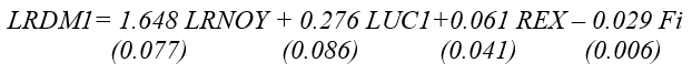
Equation (16) indicates a positive effect of the real income on the long-run money demand which is theoretically consistent. However, the opportunity cost (user cost) coefficient did not have the expected sign. Theoretically, real narrow money demand is expected to be negatively related to opportunity cost. The real exchange rate exerts a low positive influence on money demand. The foreign interest rate has the expected sign.

Table 5.6: Testing for restriction of variables in the long run relationship for the Divisia M1 model

_{Note: * indicates rejection of the null hypotheses at 5%.}

Table (5.6) presents the results of testing the restrictions on the long-run money demand variables’ coefficients. Imposing unitary restriction of the long-run income elasticity is rejected according to χ² distribution. Both user cost and foreign interest rates coefficients are statistically significant at the 5 percent level. However, we failed to reject the null hypothesis of zero coefficient of real exchange rate variable. This implies that all variables except the real exchange rate influence the behavior of the demand for Divisia M1.

c) Analysis of Simple-Sum M2 Model

The lag length of the unrestricted VAR is set to 3, based on the LR test (Likelihood Ratio Test).

Table 5.7: Johansen Maximum Likelihood test for the number of cointegrating vectors for Simple-Sum M2

Note: *(**) denotes rejection of the hypothesis at the 5 % level.

Critical values are from Osterwald-Lenum (1992).

Table (5.7) presents the results of the rank test of the Simple-Sum M2 model. It can be seen that the null hypothesis of, at most, r = 0 cointegrating vectors is strongly rejected by the data at the 5 percent significance level for both λ_-trace and λ_-max statistics. The null hypothesis of, at most, one cointegrating vector is rejected at the 5 percent significance level according to λ_-trace statistics. However, λ_-max statistics indicate that the null hypothesis of, at most, one cointegrating vector can not be rejected at the 5 percent significance level, since the calculated value of λ_-max statistics is less than its corresponding 5 percent critical value. Since the two tests’ statistics yield different results, we will follow the one that is more supported by the literature. According Johansen and Juselius (1990), λ_-trace statistics are more reliable than λ_-max statistics in a case of conflict between the two tests’ statistics. Furthermore, Cheung and Lai (1993), suggest that λ_-trace statistics are more robust than λ_-max statistics. As a result, we conclude that there exist two cointegtrating vectors for the Simple-Sum M2 model at the 5 percent significance level. Our estimated cointegrating vector is given by the eigenvector associated with the largest estimated eigenvalue.

Since our goal is to determine whether a long-run equilibrium money demand function exists between the variables, the first cointegrating vector is normalized on real money balance (Simple-Sum M2). The normalized eigenvector is given by (std.err. in parentheses)

LRSM2 = 1.949 LRNOY – 0.181 i_Riyal + 0.018 REX + 0.212Fi (5.3)

(0.09) (0.038) (0.051) (0.041)

Equation (5.3) indicates a theoretically consistent positive long run income influence on the quantity of money demanded and a negative effect of the domestic interest rate on the money demand in Saudi Arabia. However, the foreign interest rate did not have the expected signs and the real exchange rate has low positive influence on money demand.

Table 5.8: Testing for restriction of variables in the long run relationship for the

Simple-Sum M2 model

_{Note: * indicates rejection of the null hypotheses at 5%.}

Table (5.8) reports the results of testing the restrictions on the long-run money demand variables’ coefficients. Imposing unitary restriction on the long-run income elasticity is rejected according to χ² distribution. Both domestic and foreign interest rates’ coefficients are statistically significant at the 5 percent level. However, we failed to reject the null hypothesis of zero coefficient of the real exchange rate variable. This implies that all variables, except real exchange rate, influence the behavior of the demand for Simple-Sum M2.

d) Analysis of Divisia M2 Model

The lag length of the unrestricted VAR is set to 3, based on the LR test (Likelihood Ratio Test), Akaike information criterion (AIC), and Final prediction criterion (FPE).

Table 5.9: Johansen Maximum Likelihood test for the number of cointegrating vectors for Dvisia M2

Note: *(**) denotes rejection of the hypothesis at the 5 %( 1%) level.

Critical values are from Osterwald-Lenum (1992).

Trace test indicates 2 cointegrating equation(s) at 5% levels

Max-eigenvalue test indicates 1 cointegrating equation(s) at the 5% level.

Table (5.9) reports the results of the rank test of the Divisia M1 model. We can see that the null hypothesis of, at most, r = 0 cointegrating vectors is strongly rejected by both λ_-trace and λ_-max statistics at the 5 percent significance level. The null hypothesis of, at most, one cointegrating vector is also rejected at 5 percent level according to λ_-trace statistics, since the calculated value of λ_-trace statistics is bigger than its corresponding 5 percent critical value. However, according to λ_-max statistics, the null hypothesis of, at most, one cointegrating vector can not be rejected at the 5 percent significance level. It is obvious that the two tests’ statistics yield different results. However, Johansen and Juselius (1990) suggest the use of λ_-trace statistics in the situation of conflicts between the two statistics. As a result, we conclude that there exist two cointegtrating vectors for the Divisia M2 model at the 5 percent significance level.

The analysis of the cointegration relationship is based on the normalized first cointegrating vector on real money balance (Divisia M2). The normalized eigenvector is given by (std.err. in parentheses)

LRDM2 = 1.670 LRNOY + 0.131 LUC2+0.025 REX – 0.022 Fi (5.4)

(0.069) (0.054) (0.037) (0.007)

Equation (5.4) indicates a positive effect of the real income on the long-run money demand which is theoretically consistent. However, the opportunity cost (user cost) coefficient did not have the expected sign. The real exchange rate exerts a low positive influence on money demand. The foreign interest rate has the expected sign.

Table 5.10: Testing for restriction of variables in the long run relationship for the Divisia M2 model

_{Note: * indicates rejection of the null hypotheses at 5%.}

Table (5.10) presents the results of testing the restrictions on the long-run money demand variables’ coefficients. Imposing unitary restriction of the long-run income elasticity is rejected according to χ² distribution. However, the test fails to reject the exclusion of user cost, foreign interest rate, and real exchange rate variables. This implies that only the income variable influences the behavior of the demand for Divisia M2.

Cointegration Results for the Consumer Demand Theory Approach

1. Analysis of Simple-Sum M1

The lag length of the unrestricted VAR is set to 4, based on the LR test (Likelihood Ratio Test), FPE, and AIC.

Table 5.11: Johansen Maximum Likelihood test for the number of cointegrating vectors for Simple-Sum M1

Note: *(**) denotes rejection of the hypothesis at the 5 %( 1%) level.

Critical values are from Osterwald-Lenum (1992).

Table (5.11) presents the results of the rank test of the simple-sum M1 model. The results reported for the trace and maximum eigenvalue statistics show that the null-hypothesis of no-cointegrating vector linking real Simple-Sum M1 and its determinants is rejected at the 5 percent level of significance. Furthermore, both statistics reject the null-hypothesis of, at most, one cointegrating vector. However, the null-hypothesis of, at most, two cointegrating vectors is not rejected by both trace and maximum eigenvalue statistics. Thus, we conclude that there exist two cointegrating vectors for the Simple-Sum M1 model at the 5 percent significance level.

The first cointegrating vector is normalized on real money balance (Simple-Sum M1). The normalized eigenvector for the long-run money demand model of monetary aggregate Simple-Sum M1 is given by (std.err. in parentheses)

LRSM1= 0.877 + 1.878 Y + 0.116 π (5.5)

(0.07) (0.009)

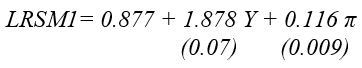
where Y is real expenditure on monetary services plus real expenditure in consumption (full income) obtained from the representative’s budget constraint, and π is the price dual (the Leontief price index). Equation 19 indicates that the income elasticity coefficient has the expected sign; however, the opportunity cost coefficient has the wrong sign.

Table 5.12: Testing for restriction of variables in the long run relationship for the Simple-Sum M1 model

Table (5.12 presents the results of testing the restrictions on the long-run money demand variables’ coefficients. Imposing unitary restriction of the long-run income elasticity is rejected according to χ² distribution. Furthermore, the exclusion of the opportunity cost variable is rejected.

b) Analysis of Divisia M1 Model

The lag length of the unrestricted VAR is set to 4, based on the LR test (Likelihood Ratio Test), Akaike information criterion (AIC), and Final prediction criterion (FPE).

Table 5.13: Johansen Maximum Likelihood test for the number of cointegrating vectors for Divisia M1

Table (5.13) presents the results of the rank test of the Divisia M1 model. The null hypothesis of zero cointegrating vectors is strongly rejected by the data at the 5 percent significance level for both λ_-trace and λ_-max statistics. However, the null hypothesis of, at most, one cointegrating vector can not be rejected as both Trace and Maximum Eigenvalue statistics are smaller than the critical values reported for each. Thus, we conclude that there exists a unique cointegrating vector for the Divisia M1 model at the 5 percent significance level.

Since there is one cointegrating vector, an economic interpretation of the long-run Divisia M1 money demand function can be obtained by normalizing the estimates of the unconstrained cointegrating vector on the real money balance (Divisia M1), which n is given by (std.err. in parentheses)

LRDM1 = – 8.64 + 1.179 Y – 0.937 π (5.6)

(0.07) (0.07)

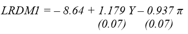
where Y is real expenditure on monetary services plus real expenditure in consumption (full income) obtained from the representative’s budget constraint, π is the price dual (user cost) for Divisia M1. Equation (20) suggests a positive and statistically significant relationship between the demand for real Divisia M1 and real income. Furthermore, the opportunity cost variable is negatively related to demand for real Divisia M1. These results are consistent with the prediction of economic theory.

Table 5.14: Testing for restriction of variables in the long run relationship for the Divisia M1 model

Table (5.14) presents the results of testing the restrictions on the long-run money demand variables’ coefficients. Imposing unitary restriction of the long-run income elasticity is not rejected according to χ² distribution. Furthermore, the exclusion of the opportunity cost variable is rejected.

c) Analysis of Simple-Sum M2

The lag length of the unrestricted VAR is set to 4, based on the LR test (Likelihood Ratio Test), FPE, and AIC.

Table 5.15: Johansen Maximum Likelihood test for the number of cointegrating vectors for Simple-Sum M2

Note: *(**) denotes rejection of the hypothesis at the 5 %( 1%) level.

Critical values are from Osterwald-Lenum (1992).

Table (5.15) presents the results of the rank test of the simple-sum M1 model. The results reported for the trace and maximum eigenvalue statistics show that the null-hypothesis of no-cointegrating vector linking real Simple-Sum M2 and its determinants is rejected at the 5 percent level of significance. Furthermore, both statistics reject the null-hypothesis of, at most, one cointegrating vector. However, the null-hypothesis of, at most, two cointegrating vectors is not rejected by both trace and maximum eigenvalue statistics. Thus, we conclude that there exist two cointegrating vectors for the Simple-Sum M1 model at the 5 percent significance level.

The estimated long-run money demand function is presented by normalizing the first cointegrating vector on real Simple-Sum M2 in the following (std.err. in parentheses)

LRSM2= 0.877 + 1.236 Y + 0.089 π (5.7)

(0.1) (0.013)

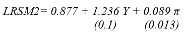
Equation (5.7) indicates that the long-run money demand for Simple-Sum M2 is determined by full income and dual price of Simple-Sum M2. The long-run income elasticity coefficient possesses the expected positive sign. However, the opportunity cost variable does not reflect the theoretically expected sign.

Table 5.16: Testing for restriction of variables in the long run relationship for the Simple-Sum M2 model

Table (5.16) presents the results of testing for restriction of variables in the long-run relationship for the Simple-Sum M2. The results suggest that the long-run income elasticity is equal to unity. Furthermore, the null hypothesis of zero coefficient of the opportunity cost variable is rejected.

d) Analysis of Divisia M2 Model

The lag length of the unrestricted VAR is set to 4, based on the LR test (Likelihood Ratio Test).

Table 5.17: Johansen Maximum Likelihood test for the number of cointegrating vectors for Divisia M2

Note: *(**) denotes rejection of the hypothesis at the 5 %( 1%) level.

Critical values are from Osterwald-Lenum (1992).

Table 17 presents the results of the rank test of the Divisia M2 model. The null hypothesis of zero cointegrating vectors is strongly rejected by the data at the 5 percent significance level for both λ_-trace and λ_-max statistics. However, the null hypothesis of, at most, one cointegrating vector can not be rejected as both Trace and Maximum Eigenvalue statistics are smaller than the critical values reported for each. Thus, we conclude that there exists a unique cointegrating vector for the Divisia M2 model at the 5 percent significance level.

Since there is one cointegrating vector, an economic interpretation of the long-run Divisia M2 money demand function can be obtained by normalizing the estimates of the unconstrained cointegrating vector on the real money balance (Divisia M2) which n is given by (std.err. in parentheses)

LRDM2 = – 7.16 + 1.379 Y – 0.779 π (5.7)

(0.03) (0.03)

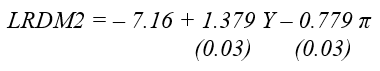
Equation (5.7) reveals a positive and statistically significant relationship between the demand for real Divisia M1 and real income. Furthermore, the opportunity cost variable is negatively related to demand for real Divisia M1. These results are consistent with the prediction of economic theory.

Table 5.18: Testing for restriction of variables in the long run relationship for the Divisia M2 model

The results presented in Table (5.18) suggest that the null-hypothesis of the long-run income elasticity equal to unity is rejected. Furthermore, the null hypothesis of zero coefficient of opportunity cost variable is rejected.

Error Correction Model Results

The finding that the variables in all different models are cointegrated means that the short-run dynamics of the relationship between them must be specified as a vector error-correction mechanism (VECM) rather than as a conventional unrestricted vector autoregression (VAR) specification. Thus, we employ a vector error correction model (VECM) to tie the short-run behavior of each money demand component to its long-run equilibrium values. The Granger Representation Theorem states that, if two or more variables are cointegrated, which means there is a long-run relationship between them, then the short-run dynamic can be described by an error-correction model.¹⁷ This can be expressed as follows:

(5.8) where and

are vector autoregressive (VAR) components in first differences and error correction components in level, respectively. X_t is 5×1 vector of monetary aggregate, non-oil GDP, opportunity cost, real exchange rate, and foreign interest rate when employing the conventional approach and is 3×1 vector of monetary aggregate, full income, and dual price when employing the consumer demand theory approach. ε_t are stationary random shocks with zero mean and constant variance. k-1 is the lag length (VAR order minus one), which is chosen by the Sequential Modified Likelihood Ratio (LR), the Final Prediction Error (FPE), the Akaike Information Criterion (AIC), the Schwarz Information Criterion (SC) and the Hannan-Quinn Information Criterion (HQ). In the case of conflicting VAR order selections, the aim is to use the one that produces the best possible results that conforms to economic theory. The presence of Granger-causality is indicated by the statistical significance of either the F-tests of joint explanatory variables or the t-tests of the error correction term (ECT). Clearly, the error correction term, which is the difference between the actual money demand and the money demand predicted by the fundamentals, plays a crucial role of self-correction mechanism of the money demand toward what is implied by the long-run determinants of the money demand function. The error-correction term must be negative and significantly different from zero. A negative coefficient on the ECT implies that, in the event of a deviation between actual and long run equilibrium level, there would be an adjustment back to the long- run relationship in subsequent periods to eliminate this discrepancy.

VECM Results for the Conventional Approach

a) Analysis of Simple-Sum M1

Δ LSM1_t = 0.0261 – 0.366Δ LSM1_t-2 – 0.142Δ LRNOY_t-1 – 0.016 Δ i_Riyal_t-1 + 0.06Δ REX_t-2

(-2.32) (-0.783) (-1.25) (1.3)

– 0.024 Δ Fi_t-1 – 0.297 EC_t-1 (5.9)

(-1.16) (-2.914)

R²= 0.31 F-statistic = [1.635] LM (1) =31.78 LM (5) = 29.38

Prob [0.16] Prob [0.24]

Portmanteau Test (3) Adj Q-Stat = 42.07 Portmanteau Test (5) Adj Q-Stat = 92.49

[0.01] [0.03]

Residual Heteroskedasticity Tests χ2 = 328.646 Jarque-Bera Normality Test = 18.76

[0.51] [0.04]

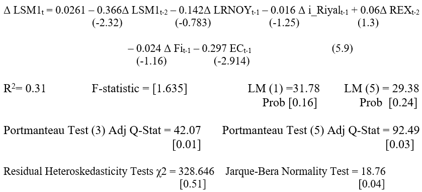
Equation (5.9) is the vector error correction model for the Simple-Sum M1 monetary aggregate where t-statistics are in parentheses and P-values in brackets. The estimated value of the error-correction term coefficient is statistically significant and has the expected sign. This implies that any excess of money held in the last period would induce to a decrease in the money holdings in the next period. However, the income coefficient did not have the expected sign and is not significant, as well as the rest of the other coefficients of explanatory variables. As for the diagnostic tests, the LM and Portmanteau Tests for serial correlation report a conflict result. Furthermore, the normality is rejected as suggested by Jarque-Bera Normality Test.

b) Analysis of Divisia M1

Δ LDM1_t = 0.029 – 0.492 Δ LDM1_t-2 – 0.339 Δ LRNOY_t-1 – 0.045 Δ UC1_t-2 – 0.046Δ REX_t-1

(5.3) (-3.4) (1.9) (-0.8) (-1.1)

– 0.025 Δ Fi_t-1 – 0.449 EC_t-1 (5.10)

(-1.6) (-5.1)

R2= 0.495 F-statistic = [3.57] LM (1) χ2 =21.29 LM (5) χ2 = 27.28

[0.50] [0.34]

Portmanteau Test (3) Adj Q-Stat = 33.07 Portmanteau Test (5) Adj Q-Stat = 96.11

[0.13] [0.05]

Residual Heteroskedasticity Tests χ2 = 340.17 Jarque-Bera Normality Test = 21.98

[0.34] [0.02]

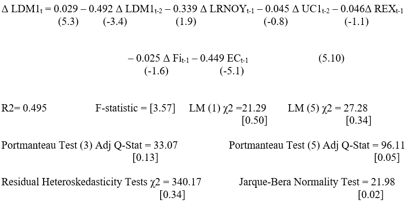
Equation (5.10) is the error correction model for the Divisia M1 monetary aggregate where t-statistics are in parentheses and P-values in brackets. The estimated value of the error-correction term coefficient is statistically significant and has the expected sign. That is, when there is excess money supply, individuals would reduce their money holdings. However, all coefficients of the explanatory variables are not statistically significant and the income coefficient did not have the expected signs. The diagnostic tests reveal no problems regarding autocorrelation, and Residual Heteroskedasticity. However, the normality is rejected, as suggested by the Jarque-Bera Normality Test.

c) Analysis of Simple-Sum M2

Δ LSM2_t = 0.015 + 0.198Δ LSM2_t-2 – 0.136Δ LRNOY_t-1 + 0.006 Δ i_Riyal_t-1 + 0.05Δ REX_t-1

(3.03) (1.19) (-1.1) (0.54) (1.84)

– 0.024 Δ Fi_t-1 – 0.043 EC_t-1 (5.11)

(-0.89) (-0.82)

R2= 0.23 F-statistic = [1.097] LM (1) χ2 =24.77 LM (5) χ2 = 20.14

[0.47] [0.74]

Portmanteau Test (3) Adj Q-Stat = 28.06 Portmanteau Test (5) Adj Q-Stat = 77.44

[0.30] [0.40]

Residual Heteroskedasticity Tests χ2 = 381.656 Jarque-Bera Normality Test = 16.35

[0.262] [0.09]

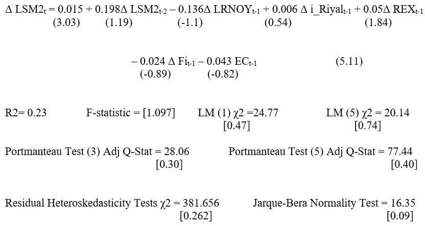
Equation (5.11) is the error correction model for the Simple-Sum M2 monetary aggregate where t-statistics are in parentheses and P-values in brackets. Although the error-correction term has the expected sign, it is not significantly different than zero. This means that the speed of adjustment towards equilibrium state does not exist. However, the diagnostic tests of the residuals show no significant evidence of autocorrelation, non-normality and hetorskedasticity. Both coefficients of the opportunity cost and the income variables do not have the expected sign and are not statistically significant.

4) Divisia M2

Δ LDM2_t = 0.03 – 0.481Δ LDM2_t-2 – 0.274 Δ LRNOY_t-1 + 0.019 Δ UC2_t-1 – 0.033Δ REX_t-1

(5.55) (-2.87) (1.74) (0.55) (-0.85)

– 0.014 Δ Fi_t-1 – 0.393 EC_t-1 (5.12)

(-1.13) (-4.83)

R2= 0.44 F-statistic = [2.94] LM (1) χ2 =24.67 LM (5) χ2 = 25.66

[0.47] [0.43]

Portmanteau Test (3) Adj Q-Stat = 31.91 Portmanteau Test (5) Adj Q-Stat = 91.36

[0.16] [0.09]

Residual Heteroskedasticity Tests χ2 = 322.77 Jarque-Bera Normality Test = 19.98

[0.60] [0.03]

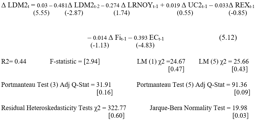
Equation (5.12) is the error correction model for the Divisia M2 monetary aggregate where t-statistics are in parentheses and P-values in brackets. The estimated value of the error-correction term coefficient is statistically significant and has the expected sign. That is, any excess of money held by economic agents in the last period would induce to a decrease in the money holdings in the next period. However, all coefficients of the explanatory variables are not statistically significant and the income coefficient did not have the expected signs. As for the diagnostic tests, the residuals show no significant evidence of autocorrelation or hetorskedasticity. However, the normality is rejected, as suggested by the Jarque-Bera Normality Test.

VECM Results for the Consumer Demand Theory Approach

a) Analysis of Simple-Sum M1

The short run Error Correction Model for Money demand is (t-statistics in parentheses and P-values in brackets):

Δ LRSM1_t = 0.0261 – 0.341Δ LRSM1_t-2 – 0.345Δ Y _t-1 – 0.027 Δ π _t-1 – 0.261 EC_t-1 (5.13)

(-2.11) (-1.98) (-2.58) (1.3) (-2.52)

R2= 0.28 F-statistic = [1.6] LM (1) =11.87 LM (5) = 5.04

[0.16] [0.83]

Portmanteau Test (4) Adj Q-Stat = 26.58 Portmanteau Test (5) Adj Q-Stat = 31.59

[0.018] [0.03]

Residual Heteroskedasticity Tests χ2 = 127.65 Jarque-Bera Normality Test (Joint) = 10.06

[0.51] [0.12]

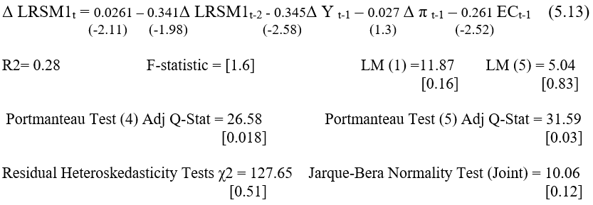
Equation (5.13) reports the short-run money demand function. The estimated value of the error-correction term coefficient is statistically significant and has the expected sign. That is, when there is excess money supply, individuals would reduce their money holdings. Although, the coefficient for the income variable is statistically significant, it has the unexpected sign. The coefficient of the opportunity cost variable has the expected sign but it is not statistically significant at the 5 percent level. Regarding diagnostic tests, no evidence of residuals hetorskedasticity is found. The Lagrang Multiplier test for one and five lags did not report any serial correlation in the residuals. However, the Portmanteau Tests reject the null-hypothesis of no serial correlation in the residuals. Furthermore, the normality is not rejected, as suggested by the Jarque-Bera Normality Test.

b) Analysis of Divisia M1 Model

The short-run Error Correction Model for Money demand is (t-statistics in parentheses and P-values in brackets):

Δ LRDM1 _t = 0.037 – 1.33 Δ LRDM1_t-1 – 1.077 Δ LRDM1_t-2 – 0.866 Δ LRDM1_t-3

(5.7) (-4.56) (-3.85) (-3.19)

+ 1.03 Δ Y _t-1 – 0.632 Δ π _t-1 – 0.498EC_t-1 (5.14)

(2.34) (2.74) (-4.24)

R2= 0.476 F-statistic = [3.63] LM (1) χ2 =8.43 LM (5) χ2 = 5.26

[0.49] [0.85]

Portmanteau Test (4) Adj Q-Stat = 11.60 Portmanteau Test (5) Adj Q-Stat = 17.46

[0.24] [0.49]

Residual Heteroskedasticity Tests χ2 = 117.45 Jarque-Bera Normality Test (Joint) = 8.54

[0.55] [0.20]

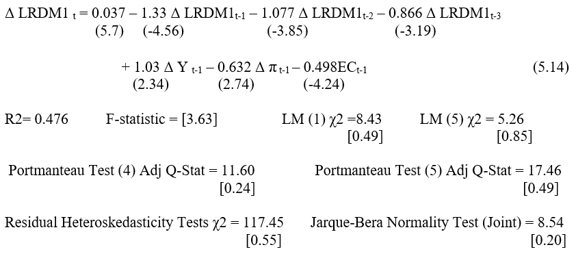
Equation (5.14) reveals a statistically significant error-correction term with an expected negative sign, indicating a valid cointegration relationship. That is, any excess of money held by economic agents in last period would induce a decrease in the money holdings in the next period. Both coefficients of the income and opportunity cost variables have signs that conform to the money demand theory. Therefore, the short-run demand for Divisia M1 seems to be influenced by lags of Divisia M1, income, and opportunity cost variables. As for the diagnostic tests, they reveal no statistical problem at all with autocorrelation, normality, and heteroskedasticity.

c) Analysis of Simple-Sum M2

The short run Error Correction Model for Money demand is (t-statistics in parentheses and P-values in brackets):

Δ LRSM2_t = 0.02 – 0.198Δ LRSM2_t-3 + 0.204Δ Y _t-2 + 0.016 Δ π _t-2 + 0.154 EC_t-1 (5.15)

(4.2) (-1.32) (2.5) (-2.00) (2.92)

R2= 0.31 F-statistic = [1.82] LM (2) =16.81 LM (5) = 7.21

[0.05] [0.62]

Portmanteau Test (4) Adj Q-Stat = 22.84 Portmanteau Test (5) Adj Q-Stat = 29.71

[0.01] [0.04]

Residual Heteroskedasticity Tests χ2 = 115.06 Jarque-Bera Normality Test (Joint) = 5.85

[0.61] [0.44]

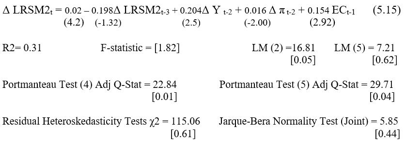
Although the error-correction term is significantly different than zero, it does not have the expected sign. This implies that the dynamic adjustment to an excess money supply by economic agents would be through increasing their demand for money, which would cause dynamic instability in the demand for money. Furthermore, only lag income would have significant influence in the money demand in the short-run. Regarding diagnostic tests, no evidence of residuals hetorskedasticity is found. The Lagrang Multiplier test for one and five lags did not report any serial correlation in the residuals. However, the Portmanteau Tests reject the null-hypothesis of no serial correlation in the residuals. Furthermore, the normality is not rejected, as suggested by the Jarque-Bera Normality Test.

d) Analysis of Divisia M2 Model

The short run Error Correction Model for money demand is (t-statistics in parentheses and P-values in brackets):

Δ LRDM2_t = 0.034 – 0.92 Δ LRDM2_t-1 – 0.73 Δ LRDM2_t-2 – 0.482 Δ LRDM2_t-3

(4.7) (-3.63) (-3.10) (-2.21)

+ 0.576 Δ Y _t-2 – 0.298Δ π 2_t-2 – 0.582EC_t-1 (5.16)

(1.87) (-1.99) (-3.35)

R2= 0.349 F-statistic = [2.15] LM (1) χ2 =12.09 LM (5) χ2 = 10.86

[0.21] [0.29]

Portmanteau Test (4) Adj Q-Stat = 10.63 Portmanteau Test (5) Adj Q-Stat = 23.16

[0.30] [0.18]

Residual Heteroskedasticity Tests χ2 = 99.67 Jarque-Bera Normality Test (Joint) = 9.69

[0.91] [0.14]

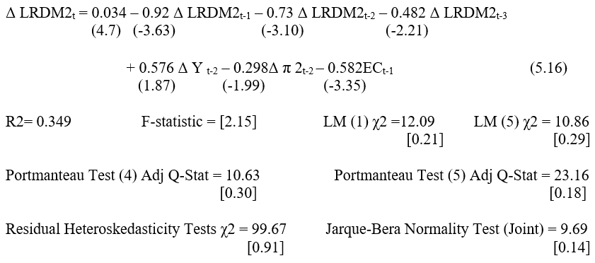
The results obtained here are very similar to those obtained when using Divisia M1. However, income and opportunity cost coefficients are not statistically significant at the 5 percent level. The estimated value of the error-correction term coefficient is statistically significant and has the expected sign. This leads to the concludsion that the short-run money demand is influenced only by lags of money. As for the diagnostic tests, they show no statistical problem at all with autocorrelation, normality, and hetorskedasticity.

Innovation Accounting Analysis

Variance decomposition and impulse response functions (IRF) are implemented to investigate and analyze the dynamic interaction in the findings. Variance decomposition analysis provides some information about the relative importance of random innovations. Variance decomposition is employed to get some information on the percentage of variation in the forecast error of a variable as explained by its own innovation, and proportion as explained by innovations in other variables in the system. The impulse response functions (IRF) indicate the transitory dynamic response of a variable to a one-standard-deviation shock to another variable. In other words, the impulse response function is a plot of the magnitude of one variable response to a one-unit change in another variable resulting from one-time shock, while keeping other variables unchanged. In analyzing the results from VDCs and IRF we discuss how the results are affected or are not affected by ordering money last or first in the VAR.

Tables (5.19) to (5.22) in the Appendix B provide results for variance decomposition of all alternative monetary aggregates, using the two alternative approaches for money demand for Saudi Arabia as attributable to their own innovations and to shocks in the other variables over a 24- quarter horizon. Tables (5.19) and (5.21) show the VDCs results when money is placed first in the VAR while tables (5.20) and (5.22) report VDCs results when money is ordered last in the VAR.

The analysis of VDCs results tend to suggest that approximately 30% to 85% of the variances in all monetary aggregates for Saudi Arabia are mainly explained by themselves, using both approaches, when money is ordered first in the VAR,. However, when ordering money last in the VAR only 3% to 38% of the variances in simple-sum M1, Divisia M1, and Divisia M2 monetary aggregates are explained by themselves, using both approaches. In regard to simple-sum M2 monetary aggregate, the ordering of money in the VAR did not affect VDCs results. In other words, the highest percentage share of the variance in simple-sum M2 monetary aggregate is mainly explained by simple-sumM2 itself regardless of the ordering of money in the VAR. Furthermore, income shocks are responsible for a significant share in the variation of all monetary aggregates excluding simple-sum M2 monetary aggregate. Income shocks account for about 14.41%, 44.42%, and 42.12% in the variance decomposition of simple-sum M1, Divisia M1, and Divisia M2, respectively, when ordering money first in the VAR and using the conventional approach. When money is placed last in the VAR Income shocks account for about 52.15%, 71.57%, and 80.72% in the variance decomposition of simple-sum M1, Divisia M1, and Divisia M2, respectively, using the conventional approach. The role of income variable in explaining the variation of the money demand function is emphasized when Divisia monetary aggregates are used as a measure for money. On the other hand, income shocks account for about 42%, 68%, 10%, and 52% in the variance decomposition of simple-sum M1, Divisia M1, simple-sum M2, and Divisia M2, respectively, when ordering money first in the VAR and using the consumer demand theory approach. When money is placed last in the VAR Income shocks account for about 85.3%, 92.98%, and 57.38% in the variance decomposition of simple-sum M1, Divisia M1, and Divisia M2, respectively, using the consumer demand theory approach. These results also confirm the importance of income variable in explaining the variation of the money demand function when Divisia aggregates are used as a measure of money.

The analysis of VDCs suggests that regardless of the ordering of money in the VAR the effect of the opportunity-cost variable is still negligible even if it is identified by the user cost when using both approaches.

In the conventional approach, two more variables also investigated the real exchange rate and foreign interest rate. Innovations to the real exchange rate account for approximately 0.37%, 2.08%, 8.15%, and 1.76 of the variances in the Simple-Sum M1, Divisia M1, Simple-Sum M2 and Divisia M2, respectively, when ordering money first. However when money is placed last, Innovations to the real exchange rate account for approximately 6.06%, 2.13%, 35%, and 1.62 of the variances in the Simple-Sum M1, Divisia M1, Simple-Sum M2 and Divisia M2, respectively.

In addition, the VDCs’ result indicates that foreign interest rate innovations can explain more of the variances in Divisia M1 and Divisia M2 than they can explain the variances of simple-sum M1 and simple-sum M2 when money is ordered first. About 22% and 14% of the variance decomposition of the Divisia M1 and Divisia M2 are explained by foreign interest rate innovations. On the other hand, foreign interest rate innovations account for less than 5% of the variance decomposition of both Simple-Sum M1 and M2, respectively. However when money is placed last, Innovations to foreign interest rate account for approximately 20%, 22%, 16%, and 14% of the variances in the Simple-Sum M1, Divisia M1, Simple-Sum M2 and Divisia M2, respectively.

Figures (5.1) through (5.16) in appendix B illustrate the IRFs of the alternative monetary aggregates from using the two alternative approaches for money demand for Saudi Arabia to one-standard-deviation innovations to all of their determinants for a 24-quarter horizon. In general and regardless of the ordering of money in the VAR, the results show that all four monetary aggregates are positively sensitive to innovations from the monetary aggregates themselves and remain strong throughout the 24-quarter horizon.

Figures (5.1), (5.2), (5.9), and (5.10) illustrate the impulse response of simple-sum M1 to shocks in its determinants. Under the conventional approach, monetary aggregate Simple-Sum M1 reacts positively to shocks to income and negatively to shocks to the opportunity-cost variable (Domestic Interest Rate) regardless of the ordering of money in the VAR. Furthermore, a shock to foreign interest rate and to real exchange rate produces a positive impact on the simple-sum M1 monetary aggregate in general under conventional approach. Under consumer demand approach, simple-sum M1 monetary aggregate react positively to shocks to income regardless of the ordering of money in the VAR. Furthermore, the simple-sum M1 monetary aggregate has no significant reaction to shocks to dual price.

Figures (5.3), (5.4), (5.11), and (5.12) illustrate the impulse response of Divisia M1 to shocks in its determinants. Under the conventional approach, monetary aggregate Divisia M1 reacts positively to shocks to income regardless of the ordering of money in the VAR. Shocks to the opportunity-cost variable (User Cost) produces a small positive effect on Divisia M1 for the first half of the 24-quarter horizon, then produces a small negative effect the second half of the 24-quarter horizon. Furthermore, a shock to the foreign interest rate produces a negative impact on the Divisia M1 monetary aggregate. Also, Divisia M1 monetary aggregates respond negatively to real exchange rate shock for the first couple periods, then shift to a positive response afterwards. The analyses of all these reactions of Divisia M1 to shocks to its determinants remain the same when changing the ordering of money. Under consumer demand approach, Divisia M1 monetary aggregate react positively to shocks to income regardless of the ordering of money in the VAR. Furthermore, the Divisia M1 monetary aggregate has almost zero response to shocks to dual price.

Figures (5.5), (5.6), (5.13), and (5.14) illustrate the impulse response of simple-sum M2 to shocks in its determinants. Under the conventional approach, when ordering money first in the VAR income shock produces a small negative effect on the simple-sum M2. However, when ordering money last in the VAR simple-sum M2 reacts positively to shocks to income. Furthermore, shocks introduced to the opportunity-cost variables (Domestic Interest Rate), foreign interest rate, and real exchange rate produce a small positive effect on the Simple-Sum M2 monetary aggregate regardless of the ordering of money in the VAR. Under consumer demand approach, simple-sum M2 reacts negatively to shocks to both income and dual price regardless the ordering of money in the VAR.

Finally, Figures (5.3), (5.4), (5.11), and (5.12) illustrate the impulse response of Divisia M2 monetary aggregate to shocks in its determinants. Under the conventional approach, monetary aggregate Divisia M2 reacts positively to shocks to income regardless of the ordering of money in the VAR. Shocks to the opportunity-cost variable (User Cost) produces a small positive effect on Divisia M2 for the first 10 periods of the 24-quarter horizon, then produces a small negative effect afterword. Furthermore, a shock to the foreign interest rate produces a negative impact on the Divisia M2 monetary aggregate. Also, Divisia M2 monetary aggregates respond negatively to real exchange rate shock for the first couple periods, then shift to a positive response afterwards. The analyses of all these reactions of Divisia M2 to shocks to its determinants remain the same when changing the ordering of money. Under consumer demand approach, Divisia M2 monetary aggregate react positively to shocks to income regardless of the ordering of money in the VAR. Furthermore, the Divisia M2 monetary aggregate has a positive response to shocks to dual price when ordering money first in the VAR and has a small negative response when ordering money last in the VAR.

Non-linear Technique (Artificial Neural Network)

The results from the Neural Network technique are presented and analyzed here. The estimations of the conventional approach for money demand using both Divisia and Simple-Sum monetary aggregates are presented first. This includes analyzing the results of the long-run money demand and short-run-adjustment money demand. The results from the second approach (the consumer demand approach) for estimating the long- and short-run money demand functions using two alternative monetary aggregates (Simple-Sum aggregates and Divisia aggregates) are presented using the same procedure of analysis used for the conventional approach. But before the results from the two approaches for money demand are discussed, the general architecture for the Artificial Neural Network used in this study is presented.

The Architecture of the Artificial Neural Network

As stated in the previous section, the BPN model, a feed-forward model, will be used to estimate the long- and short-run money demand for Saudi Arabia using both Divisia and Simple-Sum monetary aggregates. To develop the optimal network, crucial decisions must be made in designing the network. The choice of the input variables, the number of the hidden layers and hidden units, the type of activation functions in both the hidden and output layers, the value of the learning rate and the momentum rate, and the amount of training should be determined in advance. One of the shortcomings of ANN is the absence of established rules to help in choosing the optimal values of these parameters. Thus, the trial and error method is applied to obtain the appropriate values.

The input variables are chosen in accordance with the approach (conventional or consumer demand) used for estimating money demand. Regarding the number of hidden layers, it has been proven that a neural network model with one hidden layer is enough to approximate any function to any degree of accuracy (Hornik et al., 1989). However, the choice of the hidden units is rather complicated. That is, if the number of hidden units is too small, then the neural network model may not approximate the function at a desired accuracy. On the other hand, an excessive training, using too many hidden units, may result in overfitting and produce a spuriously good fit which does not lead to better forecasts. Furthermore, the greater the number of hidden layer units, the longer the training period for the network is going to be. In practice, it is very difficult to determine a sufficient number of units necessary to achieve the desired degree of approximation accuracy. Frequently, the number of units in the hidden layer is determined by trial and error. Therefore, networks with 1 to 5 hidden- layer units would be tried, and the one that produces the minimum forecast errors would be chosen.

The non-linear sigmoid function, which returns the values between zero and one, is commonly used as an activation function for the hidden layer. Following the recommendation of Rumelhart et al. (1995), the linear function is used as an activation function for the output layer. Initial weights are randomly distributed, then updated for every sample input according to the generalized delta rule, which is a specific learning rule commonly used in the back-propagation network model. Although the use of the back-propagation algorithm tends to converge slowly, it is computationally more efficient than standard optimization techniques (Manterola et al., 2002).

The number of training iterations allowed is 10,000. Using MATLAB 6.0 default values, the learning and momentum rates for the back-propagation algorithm are set to 0.01 and 0.9, respectively. Other factors that must be considered are transforming and normalizing the data into a format appropriate for neural network training to make the network more efficient. Transformation and normalization are two widely used preprocessing methods. Transformation involves manipulating raw data inputs to create a single input to a net, while normalization is a transformation performed on a single data input to distribute the data evenly and scale it so that the different input signals have approximately the same numerical range. The data would be rescaled in the range [-1, 1], which is the most common form of preprocessing to attain similar values for the data in use.

Conventional Approach to Demand for Money

Both the long-run relationship between the demand for money and its determinants and the short-run adjustment process are estimated under the conventional approach for demand for money. The long-run money demand is given by

(5.17) where NOY is non-oil GDP (scale variable), OC is the opportunity cost variable and is represented by user cost when Divisia aggregates are used and domestic interest rate when Simple-Sum aggregates are used. FI is the foreign interest rate (Eurodollar rate), and REX is the real exchange rate, which is the number of Saudi Riyal per one unit of SDR (Special Draw Rights). The following feed-forward network is used to approximate the long-run money demand relationship (φ):

(5.18)

where N_ti is the activation function (logistic function); γ₀ and γ_i are the bias term and the weight from the hidden node to output node, respectively; β_ij denotes the weight of the connection between input x_i and the jth hidden neuron; and b_i is the bias for the input x_i.

The same specification applied to the linear technique to estimate the short-run money demand function is applied here. Thus, the first difference of the real money balances is expressed as a function of its own lags, the lagged first differences of its determinants, and the lagged cointegration vector estimated from the long-run money demand. This has been done by estimating the long-run relationship first, then taking the residual as an input in the estimation of the short-run learning error-correction and adjustment process. Thus, the short-run adjustment process is

(5.19)

a) The long-run money demand results

The long-run money demand for Saudi Arabia is approximated using Divisia (M1, M2) and Simple-Sum (M1, M2) monetary aggregates. Three hidden nodes were selected for the hidden layer in the backpropagation network.¹⁸ Table (5.21) reports the goodness of fit and information criteria for Divisia (M1, M2) and Simple-Sum (M1, M2) monetary aggregates. Both R^2 and Adjusted R^2 reveal a relatively small discrepancy between the long-run Divisia (M1, M2) and Simple-Sum (M1, M2). However, Akaike, Hannan Quinn, and Schwartz Information criteria favor Divisia (M1, M2) over Simple-Sum (M1, M2). Furthermore, root mean square errors (RMSE) associated with Divisia monetary aggregates are less than those associated with Simple-Sum monetary aggregates. These variations in the RMSE are illustrated in Figures (5.9) to (5.12) (see Appendix) that plot Divisia (M1, M2) and Simple-Sum (M1, M2) monetary aggregates and their fitted values.

Table 5.21: Diagnostics of the long-run money demand for Saudi Arabia

Tables (5.22) to (5.25) (see Appendix) show the estimated weights both from input nodes to hidden nodes and from hidden nodes to output node for Divisia (M1, M2) and Simple-Sum (M1, M2). Due to the nonlinear structure of the model, these weights do not represent partial derivatives but stimulus. Thus, size of the absolute value of the weights, rather than the coefficients, is considered to assess the importance of an explanatory variable.¹⁹ According to Table (5.22), when Divisia M1 is used as a measure of money income variable (non-oil GDP), it is the most important stimulus to the hidden layer, followed by the external variable (foreign interest rate). However, both income and user-cost weights have the wrong sign. In the case of the Simple-Sum M1 monetary aggregate, income variable (non-oil GDP) is the most important stimulus to the hidden layer, followed by real exchange rate, as reported in Table (5.23). Table (5.24) shows that when the Divisia M2 monetary aggregate is used, income variable and real exchange rate are the most important stimuli to the hidden layer, respectively. However, Table (5.25) reports that when the Simple-Sum M2 monetary aggregate is used, income variable and domestic interest rate are the most essential stimuli to the hidden layer, respectively.

2. The short-run money demand results

The short-run adjustment process for Saudi Arabia is approximated using Divisia (M1, M2) and Simple-Sum (M1, M2) monetary aggregates. Four hidden nodes were selected for the hidden layer in the backpropagation network. Table (5.26) reveals the diagnostics for the approximation of the short run for Saudi Arabia using Divisia (M1, M2) and Simple-Sum (M1, M2) monetary aggregates. Contrary to the results obtained in the long-run approximation, diagnostics of the short-run money demand for Saudi Arabia favor the use of Simple-Sum (M1, M2) monetary aggregates over Divisia (M1, M2) monetary aggregates. Root mean square errors (RMSE) associated with Simple-Sum monetary aggregates are less than those associated with Divisia monetary aggregates. Furthermore, Akaike, Hannan Quinn, and Schwartz Information criteria favor Simple-Sum (M1, M2) over Divisia (M1, M2).

Table 5.26: Diagnostics of the short-run money demand for Saudi Arabia

Tables from (5.27) to (5.30) (see Appendix) show the estimated weights from both the input nodes to the hidden nodes and from the hidden nodes to the output node for Divisia (M1, M2) and Simple-Sum (M1, M2). According to Table (5.27), when the Divisia M1 aggregate is used as a measure for money, user cost (opportunity variable) is the most important stimulus to the hidden layer, followed by the external variable (Foreign Interest rate) and real exchange rate. The error-correction term has the expected sign. In the case of the Simple-Sum M1 monetary aggregate, foreign interest rate (interest on Eurodollar) is the most important stimulus to the hidden layer, followed by opportunity cost variable (domestic interest rate) and income variable (non-oil GDP), as reported in Table (5.28). The error-correction term has the expected sign. Table (5.29) shows that when the Divisia M2 monetary aggregate is used as a measure of money, income variable is the most important stimulus to the hidden layer, but the error-correction term does not have the expected sign. In the case where the Simple-Sum M2 monetary aggregate is used as a measure for money, Table (5.30) reports that the real exchange rate, followed by the foreign interest rate (interest on Eurodollar) and the domestic interest rate are the most essential stimuli to the hidden layer, respectively. Furthermore, the error-correction term has the expected sign.

Consumer Demand Approach to Demand for Money

Both the long-run relationship between the demand for money and its determinants and the short-run adjustment process are estimated under the consumer demand approach to demand for money. The long-run money demand is given by

(5.20)

where m represents Divisia (M1, M2) or Simple-Sum (M1, M2) monetary aggregates, P is the price level, Y is real expenditure on monetary services plus real expenditure in consumption (full income) obtained from the representative’s budget constraint, OC is the price dual (the Leontief price index) when m is considered as either Simple-Sum M1 or M2 monetary aggregates, and is the Divisia dual price user cost when m is considered as either Divisia M1or M2 monetary aggregates.

The following feed-forward network is used to approximate the long-run money demand relationship (φ):

(5.21)

where N_ti is the activation function (logistic function); γ₀ and γ_i are the bias term and the weight from hidden node to output node, respectively; β_ij denotes the weight of the connection between input x_i and the jth hidden neuron; and b_i is the bias for the input x_i.

The same specification applied to the linear technique to estimate the short-run money demand function is applied here. Thus, the first difference of the real money balances is expressed as a function of its own lags, the lagged first differences of its determinants, and the lagged cointegration vector estimated from the long-run money demand. This has been done by estimating the long-run relationship first, then taking the residual as an input in the estimation of the short-run learning error-correction and adjustment process. Thus, the short-run adjustment process is

(5.22)

a) The long-run money demand results

The long-run money demand for Saudi Arabia is approximated using Divisia (M1, M2) and Simple-Sum (M1, M2) monetary aggregates under the consumer demand approach. One hidden node is selected for the hidden layer in the backpropagation network. Table (5.31) reports the goodness of fit and information criteria for Divisia (M1, M2) and Simple-Sum (M1, M2) monetary aggregates. Both R^2 and Adjusted R^2 reveal a relatively small discrepancy between the long-run Divisia (M1, M2) and Simple-Sum (M1, M2). However, Akaike, Hannan Quinn, and Schwartz Information criteria favor Divisia (M1, M2) over Simple-Sum (M1, M2). Furthermore, root mean square errors (RMSE) associated with Divisia monetary aggregates are less than those associated with Simple-Sum monetary aggregates. These variations in the RMSE are illustrated in Figures (5.13 to (5.16) (see Appendix) that plot Divisia (M1, M2) and Simple-Sum (M1, M2) monetary aggregates and their fitted values.

Table 5.31: Diagnostics of the long-run money demand for Saudi Arabia

Tables from (5.32) to (5.35) (see Appendix) show the estimated weights from both the input nodes to hidden node and from hidden node to output node for Divisia (M1, M2) and Simple-Sum (M1, M2). As mentioned in the previous section, size of the absolute value of the weights rather than the coefficients is considered to assess the importance of an explanatory variable. According to Tables (5.32) and (5.34), when Divisia M1 and M2 are used as a measure of money, income variable (full income) is the most important stimulus to the hidden layer, and both income and user cost weights have the expected signs. In the case of Simple-Sum M1 and M2 monetary aggregates, income variable is the most important stimulus to the hidden layer and its weight has the expected sign. The dual price (the Leontief price index) weight has the expected sign only in the case of Simple-Sum M1, as reported in Table (5.33).

3. The short-run money demand results

The short-run adjustment process for Saudi Arabia is approximated using Divisia (M1, M2) and Simple-Sum (M1, M2) monetary aggregates. Four hidden nodes were selected for the hidden layer in the backpropagation network. Table (5.36) reveals the diagnostics for the approximation of the short-run for Saudi Arabia using Divisia (M1, M2) and Simple-Sum (M1, M2) monetary aggregates. Diagnostics of the short-run money demand for Saudi Arabia favor the use of Divisia (M1, M2) monetary aggregates over Simple-Sum (M1, M2) monetary aggregates. Root mean square errors (RMSE) associated with Divisia monetary aggregates are less than those associated with Simple-Sum monetary aggregates. Furthermore, Akaike, Hannan Quinn, and Schwartz Information criteria favor Divisia (M1, M2) over Simple-Sum (M1, M2).

Table 5:36: Diagnostics of the short-run money demand for Saudi Arabia

Tables (5.37) to (5.40) (see Appendix) show the estimated weights from both the input nodes to hidden nodes and from hidden nodes to output node for Divisia (M1, M2) and Simple-Sum (M1, M2). According to Table (5.37), when the Divisia M1 aggregate is used as a measure for money, the lags of money is the most important incentive to the hidden layer, followed by full income and user cost (opportunity variable). The error-correction term has the expected sign. The same results are obtained in the case of Simple-Sum M1 monetary aggregate. However, the error-correction term does not have the expected sign, as reported in Table (5.38). Table (5.39) shows that when the Divisia M2 monetary aggregate is used as a measure of money, the full income variable is the most important stimulus to the hidden layer and the error-correction term has the expected sign. In the case when the Simple-Sum M2 monetary aggregate is used as a measure for money, Table (5.40) reports that the full income variable is the most important stimulus to the hidden layer, followed by the price dual (the Leontief price index) as the most essential stimulus to the hidden layer. However, the error-correction term does not have the expected sign.

Conclusion

The paper states that the microeconomic theory and implies microeconomic aggregation and index number theory. It was found that money wages and hence money costs and prices of produced goods (unlike unreproducible goods such as land) tend to be sticky, certainly downwards. Considerable stickiness in the general purchasing power of money proves essential to its (and money-fixed claims) usefulness as a liquid asset and a standard for deferred payments. But this means that the system is unlikely soon to generate important (spontaneous) increases in real liquid balances. And then a very large cumulative fall in the general price level might be necessary for there to be a meaningful reduction in liquidity yields: very low carrying costs and the very generality of the uses of money, should distinguish between the possibility of land being a barrier to ultimate achievement of a positive natural interest rate and the possibility of its liquidity paralyzing or severely hampering adjustment processes requiring rapid decline in interest rates. Thus deficient aggregate demand can ensue from a collapse of expectations rather than from fundamental structural maladjustment. Of course, if the price of land is highly flexible, land is much less likely to be a drag on the system. decreases in the general price level will be necessary to reduce liquidity yields, but that sticky money costs and prices will make the rate of decline small. This can generate perverse speculative forces reducing the likelihood of lower long-term interest rates. On the other hand, if the more important liquid asset were land, Lerner argues that excess demand for liquidity would lead to rapidly-increasing land prices. The aggregate real value of land soon would satisfy demands for liquidity, eliminating excess supply in the “real” markets.

Two methods were used to analyze the dynamic interaction in our findings. The first one was the Impulse Response Function (IRF), and the second one is Variance Decomposition (VDC).it was found that non-monetary, non-reproducible assets held as liquid assets are not likely to be persistent encumbrances to full employment and growth: excess demand for these assets quickly can lead to substantial price increases until their real values have increased enough to satisfy demand. On the other hand, society is characterized by sticky money wages, at least on the down side. Excess demand for liquidity is unlikely to be corrected by spontaneous generation of additional real cash balances through price deflation of goods. Furthermore, secular deflation can set-up destabilizing expectations. Finally, the functioning of money as a liquid asset and a standard of deferred payments would be seriously impaired by thoroughgoing wage-price flexibility. Despite easy money, there can be at least two barriers to lower long rate: (a) stability of “precautionary” liquidity yield over a wide range of money-fixed holdings; (b) rigid views of “normal” short rates. And of course, gloomy prognoses of the profitability of investment in physical capital could prevent “very low” long rates from stimulating expenditure.

Non-linear Technique (Neural Network Model allowed to say that the transition from the pure theory of money to the theory of income and employment is complete. Cash is to be run down to zero at the end of each day (when payments are made to factors). But, if the receipt pattern of the representative firm is unchanged, firms will have excess cash balances most of the week unless they are able to dispose of these in the bond market. (It is assumed that households always have purchased in an even stream throughout the week. Firms will be unable to produce at planned rates without letting their cash run down. Of course, usually firms collectively pay out more in factor incomes than factors buy back from them through purchases of goods. The excess of planned output over planned purchases by factors of production is balanced by investment-expenditure plans of firms. This is what is meant by planned saving being equal to planned investment. However, firms must float securities to households if they (firms) are not to run down their cash. (Retained earnings are treated in the same way as dividends in this model.) Firms must sell securities as well as goods to households in order to maintain their cash. (“Firms” are to be interpreted as disembodied entrepreneurs who are the sole owners of physical capital. A dynamical interpretation is suggested: firms (acting independently) unable to place securities (in an ongoing situation) will cut back investment expenditures in order to protect their cash. Excess supply in the goods markets results from initial excess supply of bonds, despite the fact that ex ante saving and investment are equal.

Thus, under certainty, only the aggregate value of terminal stocks need appear in a micro criterion function. Nor would it he strictly necessary to insert financial assets under uncertainty: the criteria could concern parameters of time profiles financial assets can be viewed as means of transforming one such time profile into another, and appear (implicitly) only in the constraints. In general, money can serve as a buffer stock over the planning period guarding against shocks on current account, as a means of reducing transactions costs and illiquidity penalties as a buffer against calls or capital-account shocks. And, if short rates are not high enough to outweigh frictional expense, one would plan to hold money to meet net deficits (after bond redemptions) of short duration over any interval included in the plan. Meaningful models dealing with accumulation posit firms, here legal entities (corporations). Equities confer residual rights on shareholders. Such a model stipulates that employment of physical assets occurs within firms, implying that physical assets could not profitably (considering rents) be deployed by households. Organization and other technologies demand indirect ownership of the means of production.

The analysis of dynamic interaction in the post-sample period is investigated through innovation accounting analysis. The analysis comprises the Variance Decomposition (VDC) and the Impulse Response Function (IRF). The results from VDC and IRF indicate that the behaviors of the alternative monetary aggregates in Saudi Arabia are influenced by their determinants in all the money demand function models.The proposed model oversimplifies the financial-asset nexus. It already is implied that households manage purely financial portfolios, consumer durables having been put aside. Similarly, firms, as Management-Board decision units, largely are dealt with as deciding whether, if at all, to acquire physical assets with bonds or equities — retained earnings being imputed to equity account. In the simplest case, management, perhaps coerced by takeover-bid threats, tried to maximize net worth. Thus, lower interest rates can encourage demand for physical capital in at least two ways: effects of cheaper borrowing; effects of lower costs of equity finance to the extent that the common-share market is buoyed. it generates higher or lower demand prices for physical assets under the same circumstances as does the more sophisticated model.

Since the assumptions assure that the supply of money (bricks) is perfectly elastic within the relevant range, involuntary unemployment is impossible. If the shmoo industry does not absorb available laborers, they will turn to producing money; the money-producing activity can absorb an indefinitely large number of laborers at a wage rate (objective or shadow) of one brick per hour. This means that, if the money industry is in operation and if the labor market is perfectly competitive, the universal wage rate will be one brick per hour. The brick (money) industry can have no problem of selling output at going prices: the product itself is a perfectly general store of purchasing power. Of course, rising commodity prices would im- ply excess supply of money, indicating in turn that forces promoting involuntary unemployment had been eliminated. It would matter little if positive investment demand for money persisted over time, even if the total stock of money became indefinitely large. Persistence of high convenience yields from money balances or weakness of any wealth effects of increasing money balances is immaterial. If people want money instead of shmoos and if this lust proves insatiable, the money industry merely will continue to operate for the indefinite future. If factor and commodity prices could fall enough, any net excess supply of non-monetary commodities and factors could be accommodated by increased production of money. In sum, the new non-homogeneous system has excellent stability properties — surely if the monetized commodity is produced under nearconstant-cost conditions

The excess-demand function for money is first-order homogeneous in the m commodity prices. This is to say that the excess-demand function for real money balances is zero-order homogeneous in these prices and implies that initial excess demand for real money balances cannot be corrected by proportional reductions in commodity prices; In the real world purchase of producers’ capital involves surrender of certain sums for lottery tickets. Think of the representative lottery tickets as bearing coupons, one for each period. Each coupon can be characterized by two parameters, although an indefinitely-large number of attributes might be specified. It becomes clear why changes in interest rates (discount rates) might have little influence on the plans of entrepreneurs over the course of the business cycle. During a collapse of confidence, the elements of the yield stream might become zero or negative: regardless of the vector of non-negative interest rates. Of course partial-equilibrium analysis is limited. The demand and supply curves are mere didactic devices: numerous specifications of values for other dependent variables of the system are required. The relative price of wage goods is assumed to fall as machinery output increases. Similarly, elements of the expected future income stream depend on the profile of future outputs. And then the position of the supply curve for the machinery market will depend on the total of available resources,

The modified model is not completely satisfying intellectually, partly because we suspect that solution values for securities prices depend on the value of the wage unit. If the wage unit is reduced with output remaining the same, prices will have to fall if entrepreneurs are to be satisfied to produce at initial rates of output. Lower prices will reduce desired transactions balances, leading to excess supply of money. The deflationary effects of the higher interest rates are twofold: (a) the transitional stages find investment decreasing; (b) net investment will be lower in absolute terms at each point in time. In all of these cases prices increase with output, imposing additional pressure on the money supply. But the rate of interest must have some effect on the demand for money. In conclusion, the analyses and examinations of the long-run and the short-run of the money demand functions for all alternative measures of monetary aggregates led us to conclude that Divisia aggregates, when compared to their Simple-Sum counterparts, can serve as a potential target in formulating monetary policy in Saudi Arabia. This is explained by the fact that the Divisia aggregates provide a framework for dealing with the effects of financial innovations and also perform better at a high level of aggregation. Since Saudi Arabia is pursuing a policy of financial deregulation, which certainly will raise the competition and financial innovation in the financial industry, the use of Divisia monetary aggregates as policy instruments is recommended.

Appendix B

Table 5.19: Variance Decomposition of Forecast Errors (the Conventional Approach)

Table 5.20: Variance Decomposition of Forecast Errors

(the Conventional Approach with money ordered last)

Table 5.21: Variance Decomposition of Forecast Errors (the Consumer Demand Approach)

Table 5.22: Variance Decomposition of Forecast Errors (the Consumer Demand Approach with money ordered last)

Table 5.22: Weights for NN estimation for long-run conventional approach money demand (using Divisia M1)

Table 5.23: Weights for NN estimation for long-run conventional approach money demand (using Simple-Sum M1)

Table 5.24: Weights for NN estimation for long-run conventional approach money demand (using Divisia M2)

Table 5.25: Weights for NN estimation for long-run conventional approach money demand (using Simple-Sum M2)

Table 5.27: Weights for NN estimation for short-run conventional approach money demand (using Divisia M1)

Table 5.28: Weights for NN estimation for short-run conventional approach money demand (using Simple-Sum M1)

Table 5.29: Weights for NN estimation for short-run conventional approach money demand (using Divisia M2)

Table 5.30: Weights for NN estimation for short-run conventional approach money demand (using Simple-Sum M2)

Table 5.32: Weights for NN estimation for long-run Consumer demand approach for money demand (using Divisia M1)

Table 5.33: Weights for NN estimation for long-run Consumer demand approach for money demand (using Simple-Sum M1)

Note: OC is the opportunity cost variable (Leontief price index)

Table 5.34: Weights for NN estimation for long-run Consumer demand approach for money demand (using Divisia M2)

Table 5.35: Weights for NN estimation for long-run Consumer demand approach for money demand (using Simple-Sum M2)

Note: OC is the opportunity cost variable (Leontief price index)

Table 5.37: Weights for NN estimation for short-run consumer demand approach for money demand (using Divisia M1)

Table 5.38: Weights for NN estimation for short-run consumer demand approach for money demand (using Simple-Sum M1)

Table 5.39: Weights for NN estimation for short-run consumer demand approach for money demand (using Divisia M2)

Table 5.40: Weights for NN estimation for short-run consumer demand approach for money demand (using Simple-Sum M2)

References

Al-Badi, F. K. A. (2002). Institutional changes, money demand, and monetary policy: The case of Saudi Arabia. Unpublished Ph.D., Colorado State University, United States — Colorado.

Al-Bassam, K. A. (1990). Money Demand and Supply in Saudi Arabia: an Empirical Analysis. Unpublished Ph.D., University of Leicester (United Kingdom), England.

Al-Jasser;Muhammad, & Banafe, A. (2003). Monetary policy instruments and procedures in Saudi Arabia. Bank of International Settelments Bublications.

Anderson, R.-G., Jones, B., & Nesmith, T. (1996). Building new monetary services indices: methodology and source data. The Federal Reserve Bank of St. Louis Review, 79, 53-82.

Apostolos, S. (2001). The Demand for Money Theoritical and Empirical Approaches (1st ed.). Norwell, MA: Kluwer Academic Publishers.

Arize, A. C. (1994). A re-examination of the demand for money in small developing economies. Applied Economics, 26(3), 217.

Arize, A. C., & Shwiff, S. S. (1993). Cointegration, real exchange rate and modelling the demand for broad money in Japan. Applied Economics, 25(6), 717-726.

Bahmani-Oskooee, M. (1991). The Demand for Money in an Open Economy: The United Kingdom. Applied Economics, 23(6), 1037.

Barnett, J., and Nesmith. (1996). Divisia Second Moments: An Application of Stochastic Index Number Theory (Vol. 8). Greenwich, CT: JAI Press Inc.

Barnett, W.-A. (1978). The User Cost of Money. Economics Letters, 1, 145-149.

Barnett, W.-A. (1980). Economic Monetary Aggregates: An Application of Index Number and Aggregation Theory. Journal of Econometrics, 14, 11-48.

Barnett, W.-A. (1983). New Indices of Money Supply and the Flexible Laurent Demand System. Journal of Business and Economic Statistics, 1, 7-23.

Barnett, W. A. (1982). The Optimal Level of Monetary Aggregation. Journal of Money, Credit and Banking, 14(4), 687-710.

Barnett, W. A. (1984). Recent Monetary Policy and the Divisia Monetary Aggregates. The American Statistician, 38(3), 165-172.

Barnett, W. A. (1997). Which Road Leads to Stable Money Demand? The Economic Journal, 107(443), 1171-1185.

Barnett, W. A., Lee, Y. W., & Wolfe, M. D. (1987). The global properties of the two Minflex Laurent flexible functional forms. Journal of Econometrics, 36, 281-298.

Barnett, W. A., Offenbacher, E. K., & Spindt, P. A. (1984). The New Divisia Monetary Aggregates. The Journal of Political Economy, 92(6), 1049-1085.

Baumol, W. J. (1952). The Transactions Demand for Cash: An Inventory Theoretic Approach. Quarterly Journal of Economics, 66, 545-556.

Belongia, M.-T. (1996). Measurement Matters: Recent Results from Monetary Economics Reexamined. Journal of Political Economy, 104(5), 1065-1083.

Belongia, M.-T., & Binner, J.-M. e. (2000). Divisia monetary aggregates: Theory and practice.

Boughton, J. M. (1991a). Long-Run-Money Demand in Large Industrial Countries. IMF Staff Papers, 38, 1-32.

Brooks, C. (2002). Introductory Econometrics for Finance: Cambridge University Press.

Chauvin, Y., & Rumelhart, D. E. (1995). Backpropagation: Theory, Architectures, and Applications: Lawrence Erlbaum Associates.

Cheung, Y. W., & Lai, K. S. (1993). Finite-Sample Sizes of Johansen’s Likelihood Ratio Tests for Cointegration. Oxford Bulletin of Economics and Statistics, 55(3), 313-328.

Dahalan, J. (2003). Divisia indexes and money demand function in Malaysia. Unpublished Ph.D., Southern Illinois University at Carbondale, United States — Illinois.

Darrat, A. F. (1984). The Money Demand Relationship in Saudi Arabia: An Empirical Investifation. Journal of Economic Studies, 11(3), 43-50.

Deadman, D. F. (1995). The Demand for Money in LDCs: Empirical Results in Monetaiy Economics in Developing Countries (2^nd ed.). New York: St.Martin’s Press.

Dickey, D. A., & Fuller, W. A. (1979). Distribution of the estimators for autoregressive time series with a unit root. Journal of the American Statistical Association, 74(366), 427-431.

Dickey, D. A., & Fuller, W. A. (1981). Likelihood Ratio Statistics for Autoregressive Time Series with a Unit Root. Econometrica, 49(4), 1057-1072.

Diewert, W. E. (1974). APPLICATIONS OF DUALITY THEORY. Frontiers of Quantitative Economics: papers invited for presentation at the Econometric Society Winter Meetings, Toronto, 1972, 106.

Diewert, W. E. (1976). Exact and Superlative Index Numbers. Journal of Econometrics, 4, 115-145.

Divisia, F., &. (1925). L’indice monétaire et al théorie de la monnaie. Revue d’Economie Polittique, 39, 980-1008.

Donovan, D. J. (1978). Modeling the Demand for Liquid Assets: An Application to Canada. International Monetary Fund Staff Papers, 25, 676-704.

Dorsey, R. E., & Mayer, W. J. (1995). Genetic Algorithms for Estimation Problems With Multiple Optima, Nondifferentiability, and Other Irregular Features. JOURNAL OF BUSINESS AND ECONOMIC STATISTICS, 13, 53-53.

Enders, W. (2oo4). Applied Econometric Time Series (2nd ed.). New York: John Wiley and Sons, Inc.

Engle, R. F., & Granger, C. W. J. (1987). Co-Integration and Error Correction: Representation, Estimation, and Testing. Econometrica, 55(2), 251-276.

Ericsson, N.-R. (1998). Empirical Modeling of Money Demand. Empirical Economics, 23(3), 295-315.

Fausett, L. (1994). Fundamentals of neural networks: architectures, algorithms, and applications: Prentice-Hall, Inc. Upper Saddle River, NJ, USA.

Feenstra, R. C. (1986). Functional Equivalence Between Liquidity Costs and the Utility of Money. Journal of Monetary Economics, 17(2), 271-291.

Fisher, I. (1911). The Purchasing Power of Money. London: Macmillan.

Fisher, I. (1922). The Making of Index Numbers. Boston: Houghton Mifflin Co.

Friedman, M. (1956). The Quantity Theory of Money: A Restatement. Chicago: University of Chicago Press.

Friedman, M. (1969). The Optimum Quantity of Money and Other Essays. Chicago: University of Chicago Press.

Friedman, M. a. A. J. S. (1970). Monetary Statistics of the United States: Estimates, Source, Methods, and Data. New York: Columbia University Press (for the NBER).

Gately, E., & Gately, E. (1996). Neural networks for financial forecasting: Wiley New York.

Goldfeld, S. M., Duesenberry, J., & Poole, W. (1973). The Demand for Money Revisited. Brookings Papers on Economic Activity, 1973(3), 577-646.

Goldfeld, S. M., Fand, D. I., & Brainard, W. C. (1976). The Case of the Missing Money. Brookings Papers on Economic Activity, 1976(3), 683-739.

Goldfeld, S.-M., & Sichel, D.-E. (1990). The Demand for Money. In Handbook of MonetaryActivity Economics, 1, 299-356.

Gorman, W. M. (1959). Separable Utility and Aggregation. Econometrica, 27(3), 469-481.

Granger, C. W. J. a. R. J. (1980). An Introduction to Long-Memory Time Series Models and Fractional Differencing. The Journal of Time Series Analysis, 1, 15-29.

Hamilton, J. D. (1994). Time Series Analysis (1st ed.). Princeton, NJ: Princeton University Press.

Harb, N. (2004). Money Demand Function: Heterogeneous Panel Application. Applied Economics Letters,Taylor and Francis Journals,, vol 11(9), 551-555.

Harris, R. I. D. (1995). Cointegration Analysis in Econometric Modelling. London: Prentice Hall / Harvester Wheatsheaf.

Hebb, D. O. (1949). The Organization of Behavior: A Neuropsychological Theory: Wiley.

Hendry, D. F. (1979). Predictive failure and econometric modelling in macro-economics: The transactions demand for money. London: Heinemann.

Hendry, D. F., & Ericsson, N.-R. (1991). Modelling the demand for narrow money in the United Kingdom and the United States. European Economic Review, Elsevier, 35(4), 833-881.

Hicks, J. R. (1937). Mr. Keynes and the ‘Classics’. Econometrica, 5, 147-159

Hornik, K., Stinchcombe, M., & White, H. (1989). Multilayer feedforward networks are universal approximators. Neural Networks, 2(5), 359-366.

Johansen, S. (1988). Statistical Ananlysis of Cointegration Vecotors. Journal of Economic Dynamics and Control, Elsevier,, 12(2-3), 231-254.

Johansen, S. (1991). Determination of Cointegration Rank in the Presence of a Linear Trend. Oxford Bulletin of Economics and Statistics, 54(3), 383-397.

Johansen, S., & Juselius, K. (1990). Maximum Likelihood Estimation and Inference on Cointegration–With Application to the Demand for Money. Oxford Bulletin of Economics and Statistics, 52(2), 169-210.

Kennedy, P. (2003). A Guide to Econometrics (5th ed.). Cambridge, MA: The MIT Press.

Keynes, J. M. (1936). The General Theory of Employment, Interest, and Money. London and New York: Macmillan.

Khatib-Kswani, M. a. T., H. A.. (1999). Cointegration Error Correction and the Demand for money in Saudi Arabia. Economia-Internazionale, 52(3), 299-308.

Klein, B. (1974). Competitive Interest Payments on Bank Deposits and the Long-Run Demand for Money. American Economic Review, 64, 931-949.

Laidler, D. (1969). Money, Wealth and Time Preference in a Stationary Economy. Canadian Journal of Economics, Canadian Economics Association, 2(4), 526-535.

Laidler, D. (1993). Hawtrey, Harvard, and the Origins of the Chicago Tradition. The Journal of Political Economy, 101(6), 1068-1103.

Leontief, W. W. (1947). An Introduction to a Theory of the Internal Structure of Functional Relationships. Econometrica, 15, 361-373.

Lucas, R. E., Jr. (1980). Two Illustrations of the Quantity Theory of Money. The American Economic Review, 70(5), 1005-1014.

Lutkepohl, H. (2005). New Introduction to Multiple Time Series Analysis (1st ed.). Berlin: Springer-Verlag Heidelberg.

Lütkepohl, H., & Krätzig, M. (2004). Applied Time Series Econometrics: Cambridge University Press.

Marshall, A. (1920). Principles ofEconomics. New York, 3.

McCallum, B. T., & Goodfriend, M. (1987). Money: Theoretical Analysis of the Demand for Money. NBER Working Paper.

McCulloch, W. S., & Pitts, W. (1943). A logical calculus of the ideas immanent in nervous activity. Bulletin of Mathematical Biology, 5(4), 115-133.

McNelis, P. D., Liliana Rojas-Suárez. (1996). Money Demand, Uncertainty, and Seigniorage in Chile and Mexico: Approximation, Learning, and Estimation with Neural Networks. Interamerican Development Bank Working Paper.

Metwally, M. M., & Abdelrahman, A. M. M. (1990). The Demand for Money in the economy of Saudi Arabia. The Indian Economic Journal, 38(1), 89-102.

Miller, S. M. (1991). Monetary Dynamics: An Application of Cointegration and Error-Correction Modeling. Journal of Money, Credit and Banking, 23(2), 139-154.

Minsky, M. L. (1954). Theory of neural-analog reinforcement systems and its application to the brain-model problem. Princeton University.

Monterola, C., Lim, M., Garcia, J., & Saloma, C. (2002). Accurate Forecasting of the Undecided Population in a Public Opinion Poll. Journal of Forecasting, 21(6), 435-449.

Moshiri, S. (1998). Forecasting inflation using econometric and artificial neural network models. Unpublished Ph.D., The University of Manitoba (Canada), Canada.

Nagadi, A. H. (1985). Demand For Money in Saudi Arabia: An Empirical Study. Unpublished Ph.D., The Claremont Graduate University, United States – California.

Phillips, P. C. B. and P. Perron (1988), “Testing for a Unit Root in Time Series Regression”. Biometrika, 75, 335-346.

Phillips, P. C. B. (1987). Time series regression with a unit root. Econometrica, 55(2), 277-301.

Pigou, A. C. (1917). The Value of Money. The Quarterly Journal of Economics, 32(1), 38-65.

Qayyum, A. (2005). Modelling the Demand for Money in Pakistan. The Pakistan Development Review, Pakistan Institute of Development Economics,, vol 44(3), 233-252.

Romer, C. D., Romer, D. H., Goldfeld, S. M., & Friedman, B. M. (1990). New Evidence on the Monetary Transmission Mechanism. Brookings Papers on Economic Activity, 1990(1), 149-213.

Rosenblatt, F. (1962). Principles of neurodynamics: Spartan Books New York.

Rumelhart, D. E., Hinton, G. E., & Williams, R. J. (1985). Learning Internal Representations by Error Propagation: CALIFORNIA UNIV SAN DIEGO LA JOLLA INST FOR COGNITIVE SCIENCE.

Said, S. E., & Dickey, D. A. (1984). Testing for unit roots in autoregressive-moving average models of unknown order. Biometrika, 71(3), 599-607.

Seddighi, H., & Lawler, K. A. (2000). Econometrics: A Practical Approach: Routledge.

Serletis, A. (2001). The Demand for Money: Theoretical and Empirical Approaches: Kluwer Academic Publishers.

Sims, C. (1980). Macroeconomics and Reality. Econometrica, 48, 1-48.

Sono, M. (1961). The Effect of Price Changes on the Demand and Supply of Separable Goods. International Economic Review, 2(3), 239-271.

Soto, R. (1996). Three essays on empirical dynamics in macroeconomics. Unpublished Ph.D., Georgetown University, United States – District of Columbia.

Sriram, S. S., & International Monetary Fund Research, D. (1999). Survey of Literature on Demand for Money: Theoretical and Empirical Work with Special Reference to Error-correction Models: International Monetary Fund, Research Department.

Startz, R. (1979). Implicit Interest on Demand Deposits. Journal of Political Economy 37, 1190-1291.

Strotz, R. H. (1957). The Empirical Implications of a Utility Tree. Econometrica, 25(2), 269-280.

Sweidan, O. D. (2004). Inventories, monetary factors, and propagation of cycles. Unpublished Ph.D., Colorado State University, United States — Colorado.

Swingler, K. (1996). Applying neural networks: Academic Press London.

Tanner, E., & Devereux, J. (1993). Deficits and the Demand for Money. Southern Economic Journal, 60(2), 316-326.

Tobin, J. (1958). Liquidity Preference as Behaviour Towards Risk. Review of Economic Studies, 25, 65-86.

Vega, J. L. (1998). Money demand stability: Evidence from Spain. Empirical Economics, 23(3), 387-400.

Wankeun, O. (2002). Cointegration and structural change: An application to the U.S. demand for money. Economic Inquiry, 40(1), 91.

Barnett, William A. 1997. “Which Road Leads to Stable Money Demand?” The Economic Journal, 107:443, pp. 1171-85.

Footnotes

1. For detailed discussion of the conditions necessary for an aggregate to be optimal, see Barnett (1982).
2. The weak separability of the utility function is a necessary condition under aggregation theory. “Without the appropriate [weak] separability conditions, any aggregate is inherently arbitrary and spurious and does not define an economic variable” (Barnett, 1980, p.13).
3. Anderson, Jones, and Nesmith (1997c) prove that Divisia index exactly tracks the aggregator function in continuous time.
4. This is due to the aggregation procedure adopted by simple-sum aggregate, which gives equal weights (1) to all monetary components.
5. See Goldfeld and Sichel (1990) and Laidler (1993) for an extensive theoretical and empirical review of money demand models. See Boughton (1991a) for a review of empirical models for industrialized countries. See Deadman (1995) for a review of empirical studies for developing countries. See Ericsson (1998) for a recent review of the main methodological issues.
6. Stephen M. Goldfeld, “The Case of the Missing Money,” Brookings Papers on Economic Activity 3 (1976): 683–730.
7. Goldfeld and Sichel (1990) and Laidler (1993) provide a comprehensive review of the major theoretical and empirical issues, and cite influential studies.
8. In the absence of money illusion, an increase in the general level of prices will induce a proportionate increase in the nominal demand for money, leaving the level of real balances unchanged.
9. See Goldfeld Sichel (1990), Sriram (1999), and Serletis (2001) for a comprehensive survey on these theories.
10. See Barnett (1987) for details of the two-stage budgeting solutions.
11. Masazo Sono (1961) and Wassily Leontief (1947) laid out the definition of separability.
12. Furthermore, these government institutions are not under pressure to maximize profits.
13. See Diewert (1976, p. 21) for more details on the duality between the Simple-Sum index and the Leontief index.
14. As stated previously, benchmark asset is defined to be that asset which held solely as an investment and provide no services.
15. This test is constructed by Elliott, Rothenberg, and Stock (1996), which is based on local-to-unity asymptotic theory.
16. This means that cointegration implies the existence of the vector error correction model (VECM).
17. This means that cointegration implies the existence of vector error correction model (VECM).
18. As mentioned in the methodology chapter, one to five hidden nodes were tried in the NN system then the one with least error was chosen.
19. McNelis et.al (1996) pointed out the difficulty of assessing the statistical significance of the network weights. Instead, they suggest the use of the relative sizes of the absolute values of the network weights as measure of the relative contribution of each input to the determination of the output.